What p-Values Mean (and What They Never Meant)
A p-value is the probability of seeing data at least as surprising as yours if the null hypothesis (the boring "nothing is going on" explanation) were actually true. It is a measure of surprise, not the chance your hypothesis is right, and that single distinction clears up almost every mistake people make with it.
The p-value is the most used and most misread number in all of statistics. You have almost certainly seen one, compared it to 0.05, and called your result "significant" or not. This tutorial does the thing most guides skip: it shows you exactly what that number is by building one from scratch, then walks through the four things a p-value has never been able to tell you. Everything here uses base R, and you have already met a hypothesis test once, so you have all the background you need. You can run every block right here in your browser.
What is a p-value in plain English?
You have probably run a test and seen a line like p-value = 0.0014. You were told "below 0.05, so it is significant," and you moved on. But what is that number actually measuring? The clearest way in is an analogy you already know: a courtroom.
A court starts by presuming the defendant is innocent. In statistics, the equivalent starting assumption is the null hypothesis: the idea that nothing special is going on, that any pattern you see is just random noise. The evidence in the trial is your data. The p-value answers one precise question: if the defendant were truly innocent (if the null were true), how often would evidence look at least this incriminating just by chance? A tiny p-value means the evidence would be very surprising for an innocent defendant, so you start to doubt the innocence.
Let us make that concrete. The built-in mtcars dataset records fuel economy (mpg) and transmission type (am, where 0 is automatic and 1 is manual) for 32 cars. We will ask whether manual and automatic cars differ in mileage, using t.test(), which compares two group averages and reports a p-value.
Read the output from the bottom up. The two group means are 17.1 mpg (automatic) and 24.4 mpg (manual), a gap of about 7.2 mpg. The t = -3.7671 line summarizes that gap relative to the noise in the data, and the p-value = 0.001374 is the number we care about. In plain words: if transmission type made no real difference to mileage, a gap this large would turn up only about 14 times in 10,000 random samples. That is rare enough to make the "no difference" story hard to believe.
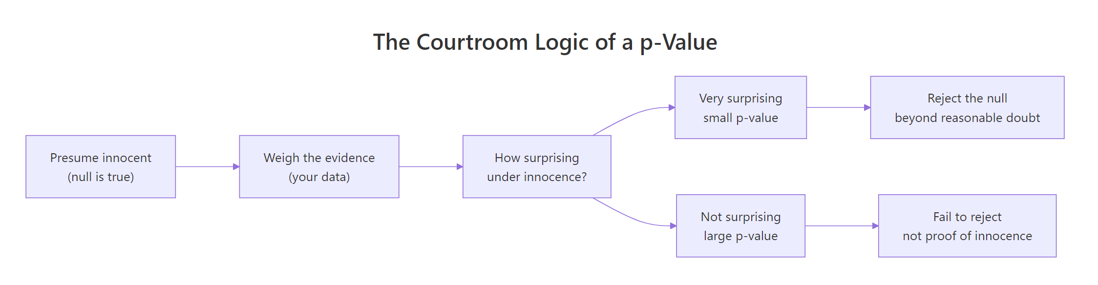
Figure 1: A p-value follows the same courtroom logic. Presume the null is true, weigh the evidence, and ask how surprising that evidence would be under innocence.
If you like the formal version, here it is. Feel free to skip this box, the sentence above is all you need.
$$p = P(\text{a test statistic at least as extreme as ours} \mid H_0 \text{ is true})$$
Where $H_0$ is the null hypothesis (no real effect), and the vertical bar means "given that" or "assuming." The whole expression is a conditional probability: it lives entirely inside the world where the null is true.
Try it: Run the same test for a different question. Do cars with a V-shaped engine differ from straight engines in mileage? Use t.test(mpg ~ vs, data = mtcars) and read off the p-value.
Click to reveal solution
Explanation: The p-value is 0.0001098, far below 0.05. A mileage gap this big between engine shapes would almost never appear if engine shape made no difference, so the "no difference" story looks unlikely.
How can you build a p-value from scratch?
Here is the part almost no tutorial shows you, and it is the part that makes everything click: you can compute a p-value yourself with nothing but shuffling and counting. No formula, no t-distribution, no memorized definition. Once you build one by hand, the phrase "assuming the null is true" stops being abstract.
The idea is simple. The null hypothesis says transmission type has no real link to mileage. So let us build that world directly: keep the mpg numbers exactly as they are, but randomly shuffle the transmission labels. Shuffling breaks any real connection, leaving only chance. If we shuffle thousands of times and measure the mpg gap each time, we get a picture of what gaps chance alone produces. Then we simply count how often chance beats our real gap.
First, we need our real, observed gap to compare against.
Manual cars average 7.24 mpg more than automatics in this sample. That is the number to beat. Now we build the null world by shuffling. We use sample() to scramble the am labels, recompute the gap, and repeat 10,000 times with replicate(). Setting a seed makes the random shuffles reproducible so your numbers match ours.
Look at what just happened. Out of 10,000 shuffled worlds where transmission was unrelated to mileage, only 5 produced a gap as large as the real 7.24 mpg. Turning that count into a proportion gives 5 divided by 10,000, which R prints as 5e-04, meaning 0.0005. That fraction is a p-value. We computed it by counting, not by any formula.

Figure 2: Building a p-value by simulation. Assume the null is true, shuffle the labels thousands of times, build the distribution of chance results, then count how many are as extreme as your real one.
Does our hand-built p-value agree with the one t.test() reported? Let us put them side by side.
Both land in the same tiny territory, well under 0.05. They are not identical to the digit, and that is fine: shuffling and the t-distribution formula are two different recipes for the same idea, and the shuffled number wiggles a little each time you change the seed or the number of shuffles. What matters is that both roads reach the same verdict, a gap this size almost never happens by chance.
It helps to see the whole null world at once. The histogram below shows all 10,000 shuffled gaps, with our real observed gap marked as a red line far out in the tail.
The pile of shuffled gaps clusters around zero, because when labels are random the two groups usually look about the same. Our real gap sits way out on the right edge, in a region chance rarely reaches. That distance is the whole story of the p-value, told as a picture.
Try it: The count of extreme shuffles is the raw ingredient of the p-value. Turn that count into a percentage, so you can say "X percent of random shuffles beat the real gap."
Click to reveal solution
Explanation: Five shuffles out of 10,000 beat the real gap, which is 0.05 percent. That small percentage is the p-value expressed on a familiar scale.
Does a p-value tell you the probability the null is true?
This is the single most common misconception, and it is worth slowing down for. Many people read p = 0.05 as "there is a 5 percent chance the null is true" or "a 95 percent chance my effect is real." Both are wrong, and the reason is subtle but important.
Look back at the definition. The p-value is the probability of your data, computed in a world where the null is assumed true. It is $P(\text{data} \mid \text{null true})$. What people want it to be is the reverse: $P(\text{null true} \mid \text{data})$, the probability the null holds given what you saw. These two are not the same, and swapping them is a classic error. Here is an everyday version: the probability the ground is wet given that it is raining is high, but the probability it is raining given that the ground is wet is much lower, because a garden sprinkler or a spilled bucket also wets the ground.
We can prove the p-value does not measure "the chance the null is true" with a quick simulation. Let us run 10,000 experiments where the null is definitely, provably true, by drawing both groups from the same population. Each group is drawn with rnorm(), which returns random numbers from a normal (bell-shaped) population with the mean and standard deviation you give it. If a small p-value really meant "the null is probably false," we should almost never see one here.
About 4.9 percent of these experiments returned p < 0.05, even though the null was true every single time. That is not a bug, it is the design: a 0.05 threshold is built to raise a false alarm 5 percent of the time when nothing is going on. So a significant result cannot mean "the null is false," because the null was true in all 10,000 of these cases and still tripped the alarm once every twenty runs.
Try it: A stricter threshold should raise fewer false alarms. Using the same true-null results in many_p, find what fraction fall below 0.01 instead of 0.05.
Click to reveal solution
Explanation: About 1 percent of true-null experiments dip below 0.01. The false-alarm rate matches whatever threshold you pick, which is exactly why the threshold is your choice, not a fact about reality.
Does a small p-value mean a big or important effect?
It is tempting to read a very small p-value as a very big effect. It does not work that way. A p-value blends together two separate things: how large the effect is, and how much data you collected. Pour in enough data and even a microscopic, meaningless effect will produce an impressively tiny p-value.
Let us watch it happen. We will fix a truly trivial effect, a difference of one-tenth of a standard deviation between two groups, and never change it. All we change is the sample size, from 50 up to 50,000 per group. The effect stays trivial the whole time; only the amount of data grows.
Read the p-value column top to bottom. At 50 per group the p-value is 0.50, nowhere near significant. At 50,000 per group it is 1.9e-53, a decimal point followed by 52 zeros before the first real digit, which is zero for any practical purpose. The effect never grew. Only the sample size did. The same tiny difference went from "invisible" to "overwhelmingly significant" purely on the strength of more data.
Try it: Where does this trivial effect cross the usual 0.05 line? Add a sample size of 200 and check its p-value.
Click to reveal solution
Explanation: At 200 per group the p-value is 0.13, still above 0.05. The same trivial effect is "not significant" at 200 and "wildly significant" at 50,000. The p-value tracks your sample size as much as your effect.
Will the same experiment always give the same p-value?
You might imagine that a real effect produces a stable, dependable p-value, so if you repeated your study you would see roughly the same number. In reality a p-value is itself a random quantity that jumps around wildly from one run to the next, even when the underlying effect never changes. Statisticians call this "the dance of the p-values."
To see the dance, we will run the same experiment twelve times. Each run compares a control group against a treatment group with a genuine, medium-sized effect built in (half a standard deviation). Nothing about the effect changes between runs. Only the random sample of 20 people per group is redrawn.
Stare at those twelve numbers. They swing from 0.002 (wildly significant) all the way up to 0.965 (utterly non-significant), and the effect was identical every single time. If you ran this study once and got 0.004, you would celebrate. Run it again and get 0.642, and you would conclude there is nothing there. Same truth, opposite verdicts, decided entirely by which 40 people you happened to sample.
So how often does this real effect actually clear the 0.05 bar? Let us run it 5,000 times and count.
Only about 33 percent of the time. This is called the study's power, and it means a genuine, medium effect studied with 20 people per group gets missed two times out of three. The effect is real in every run; the p-value simply fails to detect it most of the time because the sample is small.
Try it: Convince yourself the dance is not a fluke of one seed. Rerun the twelve studies with set.seed(99) and confirm the p-values still swing from tiny to huge.
Click to reveal solution
Explanation: A fresh seed gives a fresh dance, from 0.000 to 0.987, with the very same real effect. The p-value is a moving target, not a fixed property of the effect you are studying.
What does a p-value above 0.05 really mean?
When a p-value comes out above 0.05, people often report "there is no effect" or "the groups are the same." That is a serious mistake. A large p-value means you did not gather enough evidence to rule out chance, which is not the same as proving nothing is there. The slogan to remember: absence of evidence is not evidence of absence.
The cleanest way to see this is to build a real effect on purpose, then look at it with too little data. We know the effect exists because we put it there. Watch what a small sample does to our ability to detect it.
The p-value is 0.258, comfortably above 0.05, so a naive reading says "no effect." But we built in a real effect of 0.6, and the sample even shows it: the treatment mean (0.78) is well above the control mean (0.21). The problem is not that the effect vanished, it is that with only 10 per group we cannot separate it from noise. The confidence interval says it best. It runs from -0.46 to 1.59, meaning the true difference could plausibly be anywhere from a small reverse effect to a very large positive one. The data are consistent with almost everything, so we simply cannot conclude much.
Try it: Give the same real effect more data. Bump both groups to 40 people (keep the same means and seed) and rerun. Watch the p-value fall and the interval tighten.
Click to reveal solution
Explanation: More data pulled the p-value down from 0.258 to 0.071 and shrank the interval toward zero width. The effect was real the whole time; we just needed enough data to start seeing it clearly.
What should you report instead of just a p-value?
By now the pattern is clear: a p-value answers one narrow question and stays silent on everything else that matters. In 2016 the American Statistical Association published six principles to curb exactly the misreadings you have seen here. You do not need to memorize them, but a few plain-English rules capture the spirit and will keep you out of trouble.
- The p-value measures compatibility, not truth. It tells you how well your data fit the "nothing is going on" model, not whether that model is true.
- It is not the size or importance of an effect. A tiny p-value can sit on top of a trivial effect, as the sample-size demo showed.
- Do not worship 0.05. The 0.05 line is a convention, not a law of nature. A result at 0.049 and one at 0.051 are practically identical.
- A bare p-value is weak evidence. On its own it does not tell the reader how big the effect is or how uncertain you are.
- Always report an effect size and a confidence interval alongside it. Those answer "how big" and "how sure," the two questions the p-value ignores.
The most useful companion to a p-value is an effect size. A common one is Cohen's d, which expresses the gap between two groups in units of standard deviation, so a d of 0.5 means the groups differ by half a standard deviation. It is easy to compute by hand.
The effect size comes out to 0.39, a small-to-medium difference, and it carries a meaning a p-value never could: it says how much the groups differ, in a unit you can compare across studies. Report this next to your p-value and your reader learns both whether the signal is detectable and whether it is large enough to matter.
Try it: Practice the effect-size calculation on a bigger gap. Compute Cohen's d for two groups with means 50 and 53 and standard deviation 10, using 60 per group. The scaffold above is your model.
Click to reveal solution
Explanation: Rounded, that is the same 0.39 as before. The effect size stands on its own, no sample-size inflation, so it travels well between studies in a way a p-value cannot.
Complete Example: reading an A/B test the right way
Let us tie everything together on a realistic decision. Your team tests a new page design against the old one and measures how many minutes each visitor spends on the page. You have 400 visitors in each group. The right report is never the p-value alone; it is the p-value, the effect size, and the confidence interval, read together.
First, run the test.
The p-value is 0.00097, so the difference is unlikely to be pure chance. But we know better than to stop there. Let us gather the three numbers that actually drive the decision: the raw difference, the effect size, and the confidence interval around it.
Now read it like a professional. The new design adds about 0.21 minutes on the page, roughly 12 extra seconds. The confidence interval runs from 0.09 to 0.33 minutes and stays above zero, which is consistent with the significant p-value. The effect size is a modest d of 0.23. So the honest summary is: the improvement is real and unlikely to be chance, but it is small, and whether 12 seconds justifies shipping the redesign is a business judgment the p-value cannot make for you. That final sentence is the whole point of this tutorial.
Practice Exercises
These combine several ideas from the tutorial. Each uses fresh variable names so nothing collides with the code above. Try each before opening the solution.
Exercise 1: Estimate a false-alarm rate
Pick a significance threshold of 0.10 and estimate how often a true-null experiment falsely clears it. Simulate 10,000 experiments where both groups come from the same population (40 per group, mean 50, sd 10), collect the p-values, and compute the fraction below 0.10. Use set.seed(303) so your answer matches.
Click to reveal solution
Explanation: About 10 percent of true-null experiments fall below 0.10, matching the threshold. The false-alarm rate is simply whatever cutoff you choose, which is why the cutoff is a decision, not a discovery.
Exercise 2: Make the dance produce opposite verdicts
Take one real, fixed effect (before-mean 0.0, after-mean 0.6, sd 1, 18 people per group) and run it under two different seeds, 3 and 4. Show that the same true effect can be "significant" under one seed and "not significant" under the other, then explain why in one sentence.
Click to reveal solution
Explanation: Seed 3 gives 0.002 (significant) and seed 4 gives 0.090 (not significant), from the identical effect. The only thing that changed was which random sample of 36 people we drew, which is the dance of the p-values in a single, stark comparison.
Exercise 3: Significant but trivial
A large A/B test with 20,000 users per group finds a real difference of just 0.03 units. Run the test with set.seed(808) (both groups sd 1.2, control mean 4.00, variant mean 4.03), then report the p-value, the raw difference, the confidence interval, and Cohen's d. Decide whether you would act on this result.
Click to reveal solution
Explanation: The p-value is 0.0138, "statistically significant," yet Cohen's d is 0.0246, a practically invisible effect. This is the whole lesson in one output: significance is not importance. With 40,000 users you can detect a difference far too small to matter, so you report the effect size and walk away.
Summary
A p-value is a measure of surprise under the null hypothesis, computed by asking how often chance alone would beat your result. It is genuinely useful for one job: flagging whether a pattern is more than noise. Almost every famous misuse comes from asking it to do a different job, one it was never built for.
| A p-value IS | A p-value is NOT |
|---|---|
| The chance of data this extreme if the null were true | The chance that the null (or your hypothesis) is true |
| A measure of surprise, computed in the null world | A measure of how big or important the effect is |
| A single random draw that dances run to run | A promise about whether your study will replicate |
| Small when data are hard to explain by chance | Proof there is no effect when it is large |
The three things to carry away: build the intuition by simulation, never confuse $P(\text{data} \mid \text{null})$ with $P(\text{null} \mid \text{data})$, and always report an effect size and a confidence interval next to any p-value.
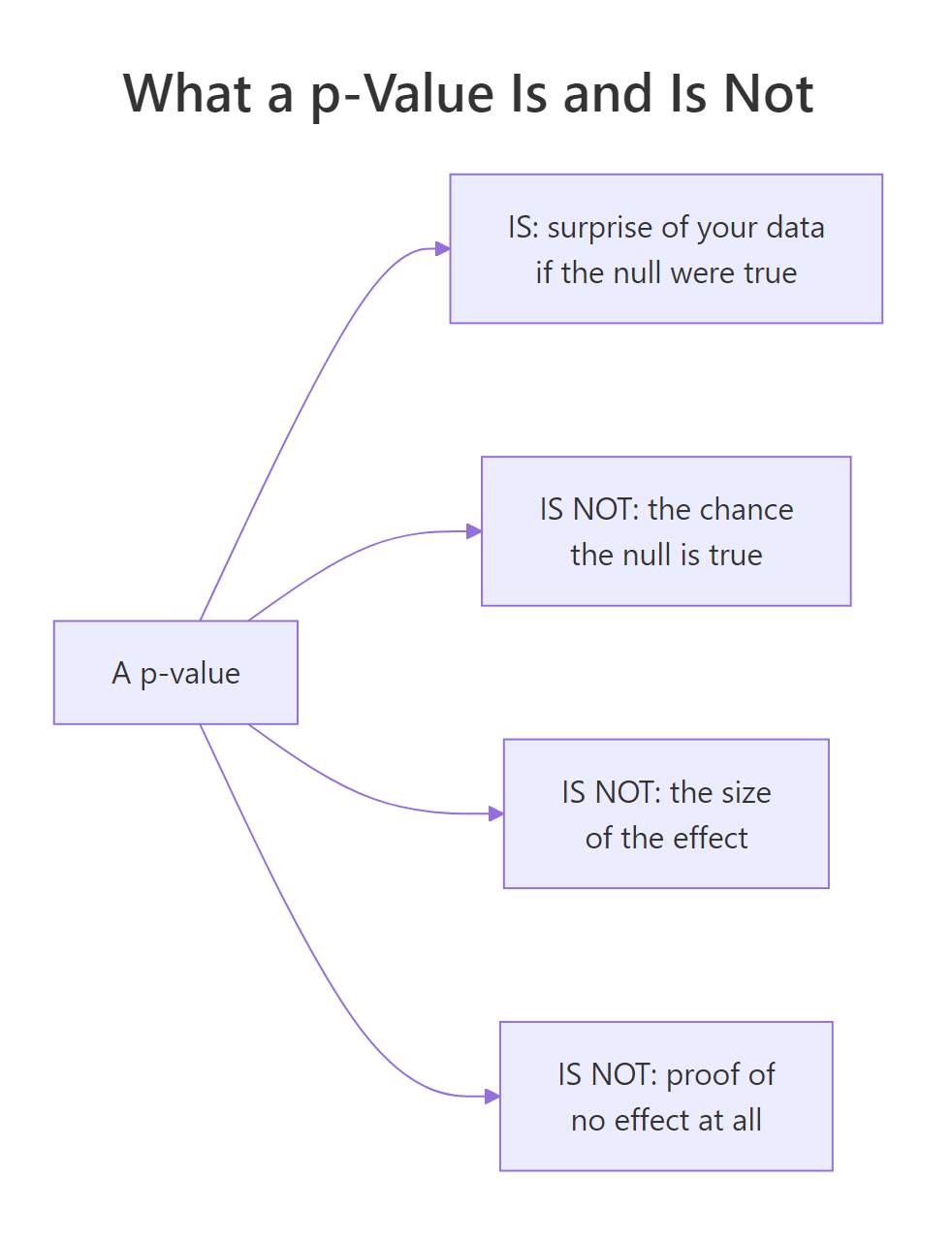
Figure 3: What a p-value is, and the three things it is not. Keep this picture in mind and most p-value mistakes disappear.
Frequently Asked Questions
Is a p-value the probability my results happened by chance? No. It is the probability of data at least as extreme as yours assuming the null (the "only chance is at work" model) is true. It starts from the chance explanation rather than measuring it.
Does a p-value below 0.05 prove my hypothesis is correct? No. As the true-null simulation showed, about 5 percent of experiments with no real effect still produce a p-value under 0.05. A small p-value is evidence against the null, not proof of your alternative.
What is a good p-value threshold to use? The 0.05 convention is a habit, not a rule. Choose your threshold before you look at the data based on how costly a false alarm is, and remember that 0.049 and 0.051 mean essentially the same thing.
If my p-value is above 0.05, can I say there is no effect? No. A large p-value means you lack the evidence to rule out chance, not that the effect is zero. Report the confidence interval so readers see which effects you actually ruled out.
What should I report alongside a p-value? Always include an effect size (such as Cohen's d) and a confidence interval. The p-value says whether an effect is detectable, the effect size says how big it is, and the interval says how sure you are.
References
- Wasserstein, R. L. & Lazar, N. A. (2016). The ASA Statement on Statistical Significance and p-Values. The American Statistician, 70(2). Link - the official statistical-association statement behind the plain-English rules in this post.
- Greenland, S. et al. (2016). Statistical tests, P values, confidence intervals, and power: a guide to misinterpretations. European Journal of Epidemiology, 31. Link - a numbered catalogue of 25 common p-value and interval misreadings, each with the correction.
- R Core Team.
t.testdocumentation, stats package. Link - the reference for every argument and output field of the function used throughout. - Cumming, G. (2014). The New Statistics: Why and How (the source of "the dance of the p-values"). Psychological Science, 25(1). Link - the paper that named the dance and makes the case for reporting effect sizes and intervals.
- Wickham, H. & Grolemund, G. R for Data Science, 2nd Edition. Link - a free, beginner-friendly grounding in the base R this tutorial assumes.
- R Core Team. An Introduction to R. Link - the canonical reference for base functions like
rnorm(),replicate(), andsample().
Continue Learning
- Your First Hypothesis Test in R: Three Ways - build a t-test three ways and see where the p-value comes from.
- Statistical vs Practical Significance in R - the effect-size side of the story, in depth.
- How Statistical Inference Works - the big picture of samples, populations, and uncertainty, with no formulas.