Your First Hypothesis Test in R: Three Ways
A hypothesis test is a simple tool for deciding whether a pattern in your data is real or just luck. In this guide you will run your very first test in R three ways, by simulation, by hand, and with a single call to t.test(), and watch all three land on the same answer.
Most tutorials hand you t.test() and move on. That teaches you the button, not the idea. Here you will build the idea first, so the button finally makes sense. We use only base R (no extra packages needed for the core work), and the built-in mtcars dataset that ships with every R install.
What question can a hypothesis test answer?
Every hypothesis test starts with a plain question about two numbers that look different. Ours: do cars with a manual gearbox get better gas mileage than cars with an automatic one? The mtcars dataset records the miles-per-gallon (mpg) and transmission type (am, where 0 means automatic and 1 means manual) for 32 cars, so let us just look at the two group averages.
The walk-through: the first two lines split the 32 cars into two piles by transmission and grab their mileage. The last line prints both averages and their gap. Manual cars average about 24.4 mpg, automatics about 17.1 mpg, a difference of roughly 7.2 mpg.
So the interpretation looks obvious: manual wins by a mile. But hold on. We only measured 19 automatics and 13 manuals. If you split any 32 cars into two random piles, the pile averages would differ a bit just by chance. A picture makes that wobble easier to feel.
Each box shows the middle half of the cars in that group, and the boxes clearly sit at different heights. But the boxes also overlap, and both groups are small. That overlap is the whole problem: is a 7.2 mpg gap big enough to trust, or is it the kind of gap random splitting could cook up on its own?
Try it: Before we go further, get comfortable pulling a group difference out of mtcars. Compute how much more (or less) horsepower (hp) manual cars have on average compared with automatics.
Click to reveal solution
Explanation: The same split-and-average recipe works for any column. The negative sign just means manual cars have less horsepower on average, not more.
What is a hypothesis test, really?
Think of a courtroom. The defendant is presumed innocent, and the prosecution has to show evidence strong enough to overturn that presumption. A hypothesis test works exactly the same way, with two competing claims.
The starting assumption is called the null hypothesis: there is no real difference, and any gap you see is just luck. The rival claim is the alternative hypothesis: the difference is real. You assume the null is true until the data makes it look ridiculous, then you reject it.
| Claim | Name | What it says here |
|---|---|---|
| Presumed true | Null hypothesis | Transmission does not affect mpg; the 7.2 gap is chance. |
| What you suspect | Alternative hypothesis | Transmission does affect mpg; the gap is real. |
To weigh the evidence you need a single number that captures "how far apart are these groups". That number is called a test statistic. And to judge whether that number is surprising, you need one more number, the most important one in the whole test: the p-value.
The p-value answers the courtroom question directly. Assuming the null hypothesis is true (no real difference), how often would pure chance produce a gap at least as big as the one you actually saw? A small p-value means "chance almost never does this", which is strong evidence against the null. A large p-value means "chance does this all the time", which is no evidence at all.

Figure 1: Every hypothesis test follows the same five steps, from question to decision.
Researchers draw the line at a threshold called the significance level, written as the Greek letter alpha, and set by convention to 0.05. If the p-value falls below 0.05, the result is called "statistically significant" and you reject the null. That 0.05 is a tradition, not a law of nature, but it is the default almost everyone starts with.
Here is the fun part. The p-value is one number, but there are several honest ways to compute it, and they agree. We will find it three ways: by shuffling the data, by plugging into a formula, and by calling one R function.
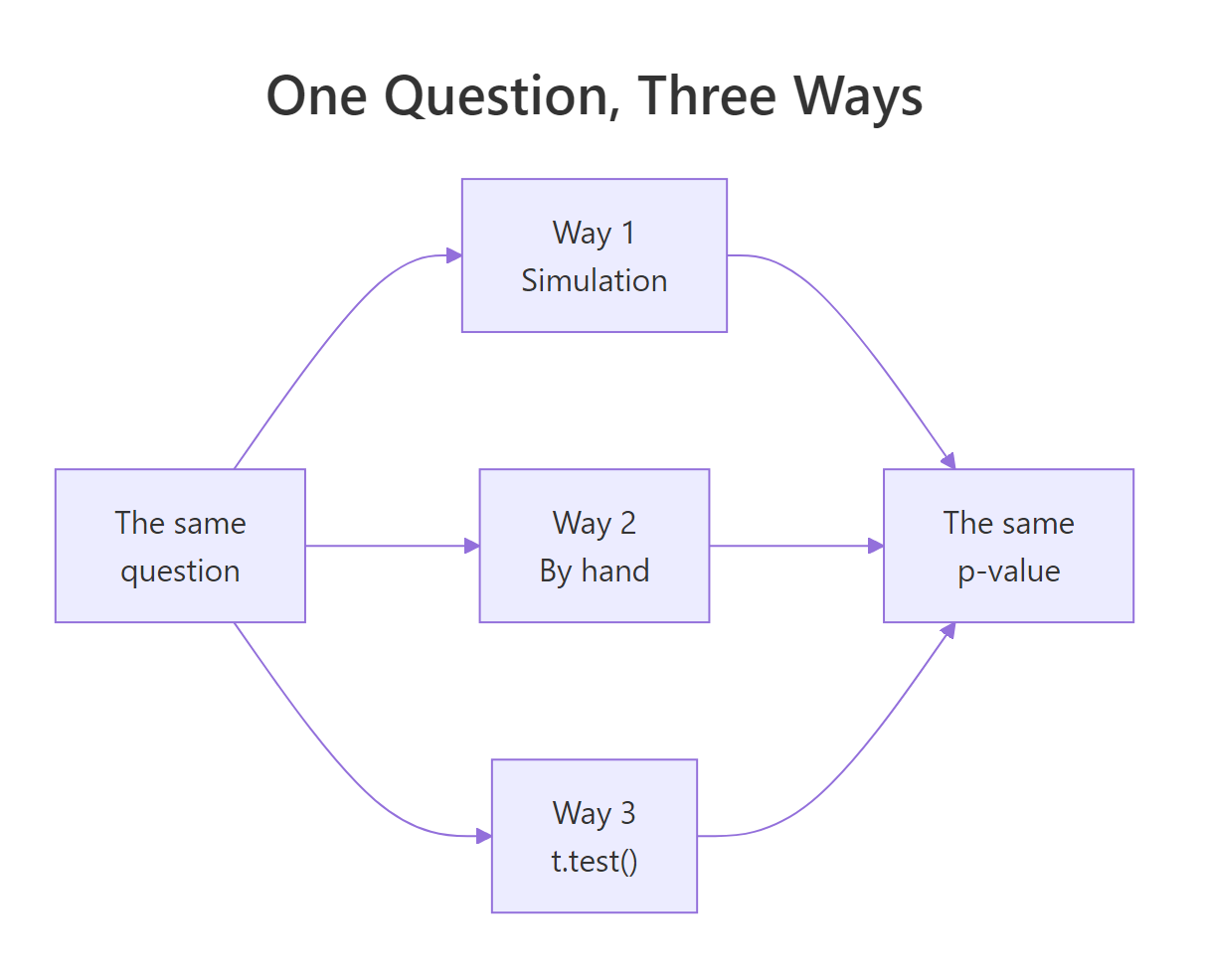
Figure 2: The same question runs through three methods and lands on one p-value.
Try it: The p-value is really just a proportion: the share of "chance" results at least as extreme as yours. Practice that idea on a tiny made-up set of gaps. If ten random gaps came out as below, what share of them are at least 3 units away from zero (in either direction)?
Click to reveal solution
Explanation: abs(ex_gaps) >= 3 gives TRUE/FALSE for each value, and mean() of TRUE/FALSE returns the proportion of TRUEs. Three of the ten values (3, 4, and -3) are at least 3 away from zero, so the share is 0.3. That proportion is exactly what a p-value is.
Way 1: Can you test it by shuffling the data?
Here is the most honest way to compute a p-value, and it needs no formulas at all. If transmission truly did not matter, then the "automatic" and "manual" labels would be meaningless stickers. We could peel them off, shuffle them, stick them back on at random, and the group gap should not change much. Let us make that idea concrete.
First, pin down the gap we are trying to explain.
Now shuffle the labels once. We take everyone's mileage, deal out the transmission labels at random, and recompute the gap. If the labels carry no real information, this shuffled gap should be small.
One shuffle gave a gap of about -2.8 mpg, much smaller than our real 7.2 and even pointing the other way. That is one draw from a world where transmission does not matter. To see the full range of what chance can do, we repeat the shuffle thousands of times and collect every gap.
replicate() just runs that shuffle-and-measure step 10,000 times and stores each result. The vector null_diffs now holds 10,000 gaps from a world where transmission is irrelevant. This collection has a name: the null distribution, the picture of what luck alone produces. Let us plot it and mark where our real gap falls.
The histogram piles up around zero, because most random label shuffles produce a small gap. The solid line marks our real gap of 7.2, and it sits way out in the empty tail where almost no shuffle reached. That visual distance is your evidence. Now turn it into the p-value by counting how many shuffles were at least as extreme as reality.
We count the shuffles whose gap was at least as far from zero as 7.2 (in either direction), then divide by the number of shuffles. The extra + 1 on top and bottom counts our real result as one more possible arrangement, which keeps the p-value from ever hitting an impossible zero. The answer is about 0.0004: out of 10,000 label shuffles, only a handful matched our gap. This test, built by shuffling, is called a permutation test.
Try it: Our count looked at gaps as big as ours in either direction, which is a two-sided test. Make it one-sided instead: count only the shuffles where manual beat automatic by at least as much as we observed.
Click to reveal solution
Explanation: Dropping abs() counts only shuffles where manual came out ahead, not shuffles that swung the other way. A one-sided p-value is smaller because it looks at just one tail of the null distribution.
Way 2: Can you test it with a formula?
Shuffling 10,000 times is intuitive, but a century ago there were no computers to do it. Statisticians found a formula that estimates the same p-value in one shot. The formula produces a test statistic called t, and the idea behind it is short: t is signal divided by noise.
The signal is the gap between the group means. The noise is a "typical" gap size you would expect from chance, called the standard error. Divide one by the other and you get a number that says how many noise-widths apart the groups are. A big t means the signal is much larger than the noise.
If you want the exact formula, here it is. If formulas are not your thing, skip to the code below, it does the same arithmetic.
$$t = \frac{\bar{x}_1 - \bar{x}_2}{s_p \sqrt{\dfrac{1}{n_1} + \dfrac{1}{n_2}}}$$
Where:
- \\( \bar{x}_1 - \bar{x}_2 \\) is the gap between the two group means (the signal)
- \\( n_1 \\) and \\( n_2 \\) are the two group sizes
- \\( s_p \\) is the pooled standard deviation, a blended measure of spread across both groups (the noise)
Let us compute t by hand so nothing is hidden. Each line matches a piece of the formula.
Reading it back: pooled_var combines how spread out each group is, se turns that spread into the size of a typical chance gap, and the final line divides our real 7.2 gap by that noise. The result, t is about 4.1, means our signal is roughly four noise-widths wide. That is large. Now we convert t into a p-value.
The function pt() reads off, from the theoretical t-distribution, how much of the tail sits beyond our t value. We multiply by 2 because the test is two-sided (a surprise in either direction counts). The df piece, short for degrees of freedom, is just a size knob for that curve, equal to the total number of cars minus 2. The p-value comes out around 0.000285, remarkably close to the 0.0004 our shuffling produced.
Try it: Reuse the exact same recipe on a different column. Compute the by-hand t-statistic comparing horsepower (hp) between automatic and manual cars.
Click to reveal solution
Explanation: A t of about -1.4 is small, so the horsepower gap is well within what chance could produce. Not every difference survives a hypothesis test, and that is exactly the point of running one.
Way 3: Can one line of R do it all?
You now understand the machinery, so you have earned the shortcut. R's built-in t.test() does every step from the last two sections in a single call. Feed it a formula, mpg ~ am, which reads as "mpg broken down by am".
Read the output top to bottom. The t = -4.1061 and df = 30 match our by-hand work exactly, and the p-value = 0.000285 matches too. The two group means at the bottom are our familiar 17.1 and 24.4. The 95 percent confidence interval line gives the plausible range for the true gap in mileage; we set it aside here and pick it up in a companion tutorial linked at the end. One line reproduced everything.
One thing to notice: our t was +4.1061 but R shows -4.1061. The sign only reflects which group R subtracts first. It puts group 0 (automatic) before group 1 (manual), so its gap is negative. The size of t and the p-value are identical, and those are what matter. We passed var.equal = TRUE so this matches our pooled by-hand formula exactly; more on R's default in a moment.
Often you do not want the whole printout, just one number to use later. Every piece is available by name.
outcome ~ group pattern powers many other R modeling functions you will meet later.If you would rather have the results as a tidy little table (handy for stacking many tests into one data frame), the broom package reshapes the output for you.
Now the promised payoff. Let us line up all three p-values side by side and confirm they tell the same story.
All three sit around 0.0003, far below the 0.05 threshold. The shuffling and the formula and the one-liner are not three different tests, they are three routes to one conclusion. That is why you can trust t.test(): you have now seen what it is doing under the hood.
Try it: Put the one-liner to work on a fresh question. Do automatic and manual cars differ in weight (wt)? Run the test and read off just the p-value.
Click to reveal solution
Explanation: The p-value is about 0.00001, far below 0.05, so automatic and manual cars clearly differ in weight too. Chaining $p.value onto the call grabs the single number without printing the full report.
How do you read and report the result?
You have a p-value of about 0.0003. The decision rule is mechanical: compare it to your significance level of 0.05. Since 0.0003 is smaller, you reject the null hypothesis and call the difference statistically significant. There is strong evidence that transmission type really is linked to mileage.
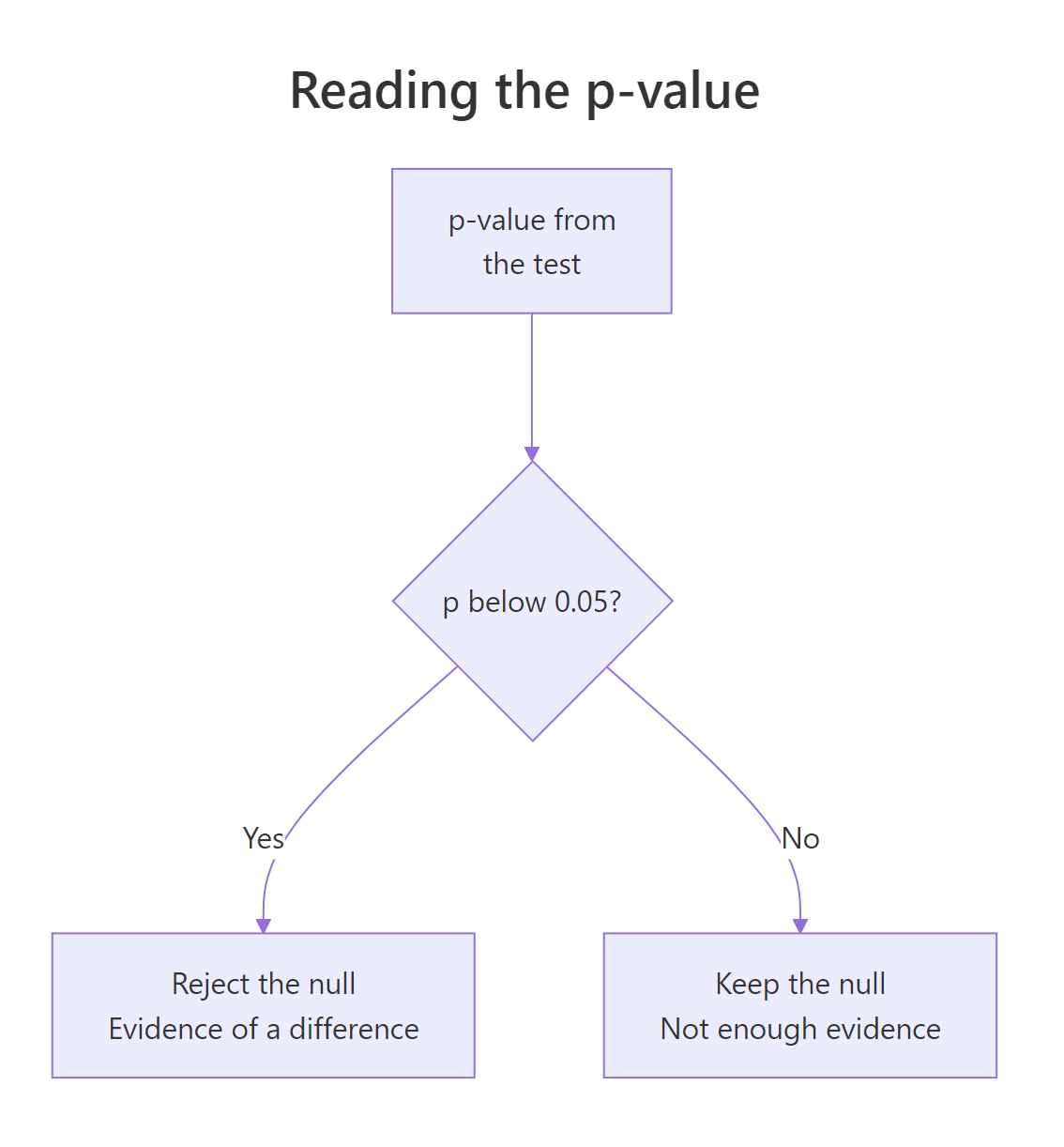
Figure 3: Compare the p-value to 0.05 to reach a decision.
Now the single most important warning in all of statistics, because almost everyone gets this wrong at first.
A p-value also says nothing about how big or important the effect is, only how surprising it is. With enough data, a tiny, meaningless difference can earn a tiny p-value. So always report the actual size of the gap alongside the p-value. A common size measure is Cohen's d, which expresses the gap in units of the data's own spread.
A rough reading guide: d near 0.2 is small, 0.5 is medium, and 0.8 is large. Our d of about 1.48 is very large, so the mileage gap is not just statistically significant, it is big enough to matter to a real car buyer. That is the difference between statistical significance and practical significance, and you should always check both.
One more honest detail. We used var.equal = TRUE, but R's default is a slightly safer version called Welch's test, which does not assume the two groups have equal spread. Here is what the default gives.
var.equal = TRUE and you get it automatically. We only forced the pooled version so it would line up with the hand formula.Two quick housekeeping notes before you go. First, choose one-sided or two-sided before you look at the data: use two-sided (the default) when a difference in either direction is interesting, and one-sided (alternative = "less" or "greater") only when you genuinely care about one direction. Second, the t-test assumes the observations are independent and roughly bell-shaped; if your data is heavily skewed or full of outliers, reach for a rank-based test like the Wilcoxon test or lean on the permutation approach from Way 1.
Try it: You already know weight differs between groups (tiny p-value). But how big is that effect? Compute Cohen's d for weight (wt) by transmission.
Click to reveal solution
Explanation: A d of about -1.9 is enormous (manual cars are far lighter), which fits the near-zero p-value you found earlier. The negative sign just reflects the direction; the magnitude is what tells you the effect is huge.
The whole test in one script
In practice you will not shuffle or hand-crank the formula every time. Once you trust t.test(), a complete, reportable hypothesis test is just a handful of lines: run the test, measure the effect size, and state the conclusion in plain words.
That block is a template you can reuse for any two-group comparison: swap in your own outcome and grouping column, and it reports the gap and its p-value, then the effect size and a plain verdict.
Practice Exercises
Work through these to lock in the ideas. Each builds on the tools above. Try to write the code before opening the solution.
Exercise 1: A one-sample test
So far we compared two groups. t.test() can also compare one group against a fixed number. Test whether the average mileage of all 32 cars is different from 20 mpg.
Click to reveal solution
Explanation: The p-value is 0.93, far above 0.05, so you keep the null. The average mpg (about 20.1) is not meaningfully different from 20. This is a result that fails to reject, which is just as valid an outcome as rejecting.
Exercise 2: The same question, two ways
Do 4-cylinder cars get different mileage than 6-cylinder cars? Answer it twice, once with a permutation test and once with t.test(), and confirm the two p-values agree.
Click to reveal solution
Explanation: Both routes land near 0.0013, comfortably below 0.05, so 4-cylinder cars really do get better mileage than 6-cylinder cars. Once again the shuffle and the formula agree.
Exercise 3: One-sided test plus effect size
Combine three ideas. Run a one-sided test asking specifically whether manual cars beat automatics, compute Cohen's d for the same comparison, and write a one-sentence conclusion.
Click to reveal solution
Explanation: The one-sided p-value (0.00014) is half the two-sided one because it only looks at one tail. With a p-value far below 0.05 and a very large effect size (d of about 1.5), you can conclude that manual cars get substantially better mileage than automatics in this dataset.
Frequently Asked Questions
What is the difference between a t-test and a hypothesis test?
A hypothesis test is the general procedure: state a null hypothesis, compute a p-value, then decide. A t-test is one specific hypothesis test, the one you use to compare means. There are many other tests (chi-square for counts, ANOVA for three or more groups) that follow the same procedure with a different test statistic.
What does the p-value actually tell me?
It tells you how compatible your data is with the null hypothesis. A small p-value means your data would be very unusual if the null were true, which is evidence against the null. It does not tell you the probability that the null is true, nor how large the effect is.
Should I use var.equal = TRUE or the default Welch test?
Use the default (Welch). It does not assume the two groups have equal spread, so it is safe in more situations, and the cost when spreads happen to be equal is negligible. We only set var.equal = TRUE in this tutorial so the one-liner would match the hand-computed formula exactly.
What if my data is not normally distributed?
The t-test tolerates mild departures from normality, especially with larger samples. For heavily skewed data or small samples with outliers, use a permutation test (Way 1 in this article) or a rank-based test such as the Wilcoxon test, both of which avoid the bell-curve assumption.
Is a small p-value the same as a big, important effect?
No. A p-value measures surprise, not size. With a large enough sample, a trivial difference can produce a tiny p-value. Always report an effect size, such as Cohen's d, next to the p-value so readers can judge whether the difference actually matters in practice.
Summary
You learned what a hypothesis test really is and ran your first one three different ways, watching all three agree.
| Way | What it teaches | The R tool | When to reach for it |
|---|---|---|---|
| Simulation | What a p-value truly means | sample() and replicate() |
Small or messy data; building intuition |
| By hand | The signal-over-noise formula | var(), pt() |
Understanding what the function computes |
| One line | The fast, standard workflow | t.test() |
Everyday analysis |
Key takeaways to carry forward:
- The null hypothesis assumes no real difference; a p-value measures how often chance alone would beat your data if the null were true.
- Reject the null when the p-value falls below your significance level (0.05 by convention).
- A p-value is not the probability the null is true, and it does not measure effect size, so always report a size measure like Cohen's d too.
- Prefer the Welch
t.test()default in real work, and switch to a permutation or rank-based test when your data is far from bell-shaped.
References
- R Core Team. An Introduction to R, section on statistical models and tests. Link
- R Documentation.
t.testfunction reference (the stats package). Link - Wickham, H. and Grolemund, G. R for Data Science, 2nd Edition. O'Reilly (2023). Link
- Diez, D., Barr, C. and Cetinkaya-Rundel, M. OpenIntro Statistics, 4th Edition, chapter on inference and randomization tests. Link
- Ismay, C. and Kim, A. Statistical Inference via Data Science (ModernDive), simulation-based inference. Link
- Cohen, J. Statistical Power Analysis for the Behavioral Sciences, 2nd Edition. Routledge (1988).
- broom package documentation, tidying model outputs. Link
Continue Learning
- Hypothesis Testing in R: a wider tour of tests beyond the t-test, including chi-square and ANOVA, once you are comfortable with the basics here.
- Confidence Intervals in R: the natural companion to the p-value, showing the plausible range for the true difference rather than a single yes-or-no verdict.
- Wilcoxon, Mann-Whitney and Kruskal-Wallis in R: the tests to reach for when your data is skewed and the t-test's assumptions do not hold.