Populations, Samples and Sampling Bias in R
A population is the whole group you want to draw a conclusion about, and a sample is the smaller slice you actually measure. Sampling bias is when the way you pick that slice systematically pushes your answer away from the truth, and unlike ordinary random noise, collecting more data does not fix it.
Almost every number you read, from an election forecast to a drug's success rate, comes from a sample, not from measuring everyone. That makes one question the quiet foundation of all of statistics: does the slice you measured actually stand in for the whole group? This lesson answers it from scratch. We will build a whole make-believe town in R so we know the real answer, take samples from it, and watch exactly when a sample reflects the town and when it misses. We use plain base R throughout, so there is nothing to install.
What is the difference between a population and a sample?
You almost never get to measure everyone. To learn the average height of a city, you do not line up two million people, you measure a few hundred and generalize from them. The whole group you care about is the population, and the handful you measure is the sample. Let's make this concrete by inventing a town where we secretly know every single height, then taking a sample and seeing how close it lands.
We will create 50,000 residents, each with a gender and a height in centimeters. Because we build every resident ourselves, we can compute the town's true average height, the number a real researcher could never see. Then we draw 100 people at random and average just them. Run the block and compare the two numbers.
Reading the two lines from top to bottom, the true average height across all 50,000 residents is 168.45 cm. The average of a random 100-person sample is 169.07 cm. They are not identical, but they are strikingly close, and we got the second number by measuring only 1 person in 500.
That gap of about half a centimeter is the price of not measuring everyone, and it is small precisely because we chose the 100 people at random. This is the core promise of sampling: a well-chosen sample stands in for the population well enough to answer the question. The diagram below is the mental model for the rest of the lesson.
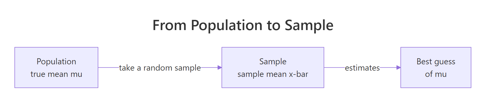
Figure 1: A statistic from a random sample is our best guess at the population parameter we cannot measure directly.
Before going further, it helps to name the pieces. Let's peek at the raw data so the words attach to something you can see.
Each row is one resident, our sampling unit, and there are 50,000 of them in total. The full set of 50,000 rows is the population. A sample is any subset of those rows, like the 100 we drew above. In a real study you would never hold this whole table, you would only ever see the sampled rows and have to reason back to the town.
Two more terms make the picture complete. The target population is the group you actually want to conclude about, here every adult in the town. The sampling frame is the list you draw from in practice, like a phone directory or a customer database. When the frame leaves people out, trouble starts, and we will return to exactly that later.
Try it: Take your own random sample of 30 residents from population and compute their average height. It should land near the true 168.45 cm.
Click to reveal solution
Explanation: sample(nrow(population), 30) picks 30 random row numbers, and we average the height column of just those rows. The result, 170.57 cm, is close to the true 168.45 cm but a bit further off than the 100-person sample was. Smaller samples wobble more, an idea we make precise soon.
What is the difference between a parameter and a statistic?
Now that you can tell a population from a sample, there is a matching pair of words for the numbers you compute from each. A number that describes the whole population is a parameter. A number computed from a sample is a statistic. The average height of all 50,000 residents is a parameter; the average of your 100-person sample is a statistic.
The distinction matters because of one asymmetry: a parameter is a fixed fact about the population that you usually cannot see, while a statistic is something you can always compute from your data. Statistics exist to estimate parameters. Let's compute the town's parameters first, since we are lucky enough to have the whole population.
The population has 50000 members, a mean height of 168.45 cm, and a standard deviation of 9.17 cm, which measures how spread out the heights are. These three numbers are parameters: they describe the entire town and they never change, because the town never changes. In statistics we give them Greek letters, \(N\) for the size, \(\mu\) (mu) for the mean, and \(\sigma\) (sigma) for the standard deviation.
Now the same summaries computed from a single 100-person sample. These are statistics, and we mark them with ordinary Roman letters to keep them straight.
This sample has \(n = 100\) people, a sample mean of 168.55 cm, written \(\bar{x}\) (x-bar), and a sample standard deviation of 9.82, written \(s\). Each statistic sits close to its matching parameter: 168.55 estimates the true 168.45, and 9.82 estimates the true 9.17. That is a statistic doing its job, standing in for a parameter it cannot see directly.
sd(). The two nearly agree once the sample is large.Here is the full notation you will meet everywhere in statistics. Greek letters are the hidden truths; Roman letters are what you compute from data.
| Quantity | Population parameter | Sample statistic |
|---|---|---|
| Size | \(N\) (everyone) | \(n\) (how many you measured) |
| Mean | \(\mu\) (mu) | \(\bar{x}\) (x-bar) |
| Standard deviation | \(\sigma\) (sigma) | \(s\) |
| Proportion | \(P\) | \(\hat{p}\) (p-hat) |
Try it: Roughly half the town is men. Compute the population proportion of men (the parameter \(P\)), then the proportion of men in a random 200-person sample (the statistic \(\hat{p}\)).
Click to reveal solution
Explanation: A logical test like gender == "men" becomes TRUE/FALSE, and averaging it gives the fraction that are TRUE. The true proportion \(P\) is 0.499, and the sample estimate \(\hat{p}\) is 0.515, close but not exact, just like the mean.
Why does a random sample represent the population?
You have now seen a few samples land near the truth, but why should you trust that to keep happening? The honest answer is that any single sample can miss. What saves us is the pattern across many samples. Let's draw not one sample but a thousand, record each one's mean, and study the whole collection.
We repeat the same action a thousand times: pick 100 residents at random and store their mean height. This gives us 1,000 sample means to look at together. The replicate() function does the repeating for us.
Look at the first two numbers. The true population mean is 168.45, and the average of our 1,000 sample means is 168.47, almost exactly the same. Individual samples scatter, but they scatter evenly around the truth, so their average lands right on it. This is what we mean when we say random sampling is unbiased: it has no built-in tendency to run high or low.
The third number, 0.97, is the standard deviation of those sample means, a measure of how much a typical sample mean strays from the truth. That spread is exactly the sampling error: the ordinary, expected wobble that comes from measuring a sample instead of everyone. A picture makes the pattern obvious.
The histogram is a tidy mound centered on the red line, which marks the true mean. Most sample means fall within about a centimeter of the truth, and extreme misses are rare. This mound shape, called the sampling distribution, is why a single random sample is usually a safe bet.
If sampling error is just random wobble, then a bigger sample should wobble less. Let's test that by repeating the experiment with 400 people per sample instead of 100.
The spread drops from 0.97 at 100 people to 0.47 at 400 people, roughly cut in half. Quadrupling the sample size halved the error, which is the general rule for sampling error. Bigger samples buy you tighter, more reliable estimates.
Try it: Repeat the thousand-sample experiment with a tiny sample size of 25 and report the spread. It should be larger than the 0.97 you saw at size 100.
Click to reveal solution
Explanation: With only 25 people per sample, the spread jumps to 1.8, nearly double the 0.97 we got at 100. Smaller samples carry more sampling error, which is the flip side of the rule that bigger samples carry less.
What is sampling bias, and how is it different from sampling error?
So far every sample has centered on the truth, because we always chose people at random. Now we break that. Suppose you collect heights at a men's sports club, so every person you measure happens to be a man. Your method is no longer neutral, and this is where sampling bias enters. Let's run the thousand-sample experiment again, but draw only from men.
The code mirrors the earlier simulation, with one change: we first find the row numbers of all the men, then sample only from them. Everything else is the same, so any difference in the result comes purely from the biased selection.
The three numbers tell the whole story. The truth is 168.45. Our earlier random method estimated 168.47, essentially perfect. The men-only method estimates 174.89, more than 6 cm too high, every single time. That consistent overshoot in one direction is bias, and it is a completely different animal from the random wobble of sampling error.
Here is the part that surprises people. With random sampling, more data fixed the error. Does more data fix bias too? Let's rerun the biased method with 1,000 people per sample instead of 100.
Growing the sample tenfold changed the biased estimate from 174.89 to 174.91. It did not move toward the truth at all; it just became a more precise wrong answer. This is the single most important idea in the lesson: sampling error shrinks as your sample grows, but sampling bias does not. The figure below contrasts the two.
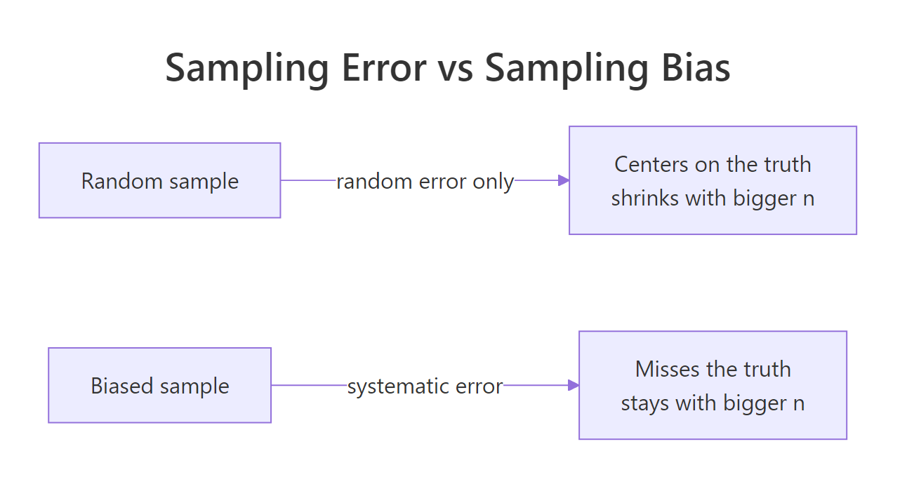
Figure 2: Random error scatters around the truth and shrinks with n; bias sits off to one side and stays.
Try it: Push the biased sample size even higher, to 2,000 men per sample, and confirm the estimate is still stuck near 175, nowhere near the true 168.45.
Click to reveal solution
Explanation: Even at 2,000 people per sample, the biased estimate holds at 174.91, still about 6 cm above the true 168.45. The bias is baked into the selection method, so no sample size can wash it out.
What are the common types of sampling bias?
Sampling bias is not one thing, it is a family of ways your selection can systematically miss. Knowing the named types helps you spot them before they wreck a study. The table lists the five you will meet most often, each with a plain-English mechanism and an everyday example.
| Type of bias | What goes wrong | Everyday example |
|---|---|---|
| Selection (convenience) | You sample whoever is easy to reach | Surveying shoppers at one upscale mall |
| Voluntary response | Only people who opt in are counted | An online poll only strong opinions answer |
| Undercoverage | The frame leaves out a whole group | A phone survey that misses people without phones |
| Nonresponse | Those who refuse differ from those who answer | A health survey the sick skip |
| Survivorship | You only see the ones that made it | Rating a strategy using only funds that still exist |
Let's implement two of these in real code, so you can see the distortion, not just read about it. First, voluntary response bias. Imagine a "height study" people opt into, where taller people are prouder of their height and more likely to volunteer. We model that by making the chance of responding rise with height.
We gave each resident a response chance that climbs with their height, then kept only the 4547 who volunteered. The last line does the selecting: runif(N) draws a random number between 0 and 1 for each resident, and keeping those below p_respond admits each person with exactly their own response chance. Their average height is 171.26 cm, nearly 3 cm above the true 168.45. Nobody lied and nothing was mismeasured; the sample tilted high simply because taller people were likelier to raise their hands.
Now survivorship bias, the easiest of the five to overlook. Suppose you study "the height of professional models" and only the very tall ever make the cut, so shorter people never appear in your data at all. We mimic that by keeping only residents above 178 cm.
By looking only at the 8244 residents who cleared the 178 cm bar, the average shoots up to 182.60 cm, a full 14 cm above the truth. The people who did not "survive" the selection are invisible, so they cannot pull the average back down. The mindmap gathers all five types in one view.
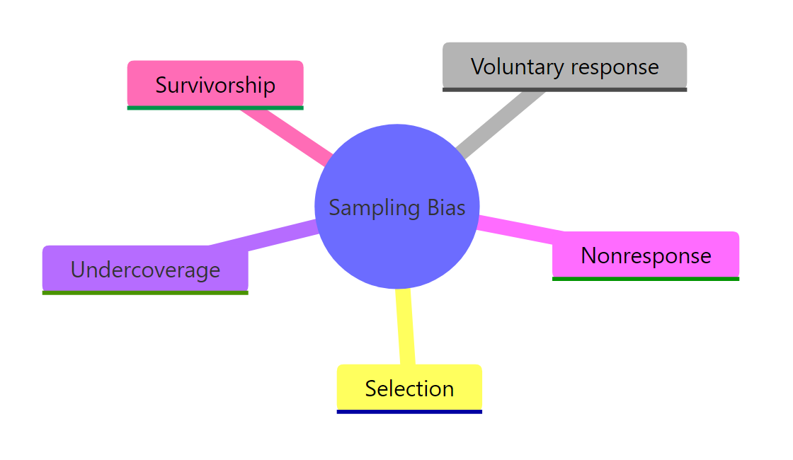
Figure 3: Five common ways a sample stops representing its population.
Try it: Model nonresponse bias. Give residents taller than the mean a 0.9 chance of responding and shorter ones only 0.3, then compare the respondents' average height to the truth.
Click to reveal solution
Explanation: Because taller residents answered far more often, the respondent average climbs to 172.25 cm, well above the true 168.45. Nonresponse bites whenever the people who skip your survey differ from the people who answer it.
How can you reduce sampling bias in practice?
The good news is that bias is a property of your method, so a better method removes it. The single most powerful fix is probability sampling: give every member of the population a known, non-zero chance of being picked, most simply an equal chance for everyone. That is a simple random sample, and R's sample() function does it directly.
A quick way to check whether a sampling method is fair is to compare a known feature of your sample against the same feature in the population. We know the town is about half men, so a fair 500-person sample should be too. Let's verify.
The population is 0.499 men and 0.501 women, and our random sample is 0.512 men and 0.488 women, a near-perfect match. Because we selected at random, the sample inherited the town's makeup automatically. Contrast that with the men-only method from before, which would have shown 1.000 men, an instant red flag that the sample does not represent the town.
Beyond random selection, three habits keep bias low in real studies. Define your target population and sampling frame carefully so no group is quietly excluded. Chase down nonrespondents with reminders, since the people who skip surveys are usually the ones who differ most. And benchmark your sample against facts you already know, like census age or gender splits, to catch a lopsided sample early. For the deeper toolkit of stratified, cluster, and systematic designs, see the companion tutorial on sampling methods.
Try it: Draw your own random 500-person sample and confirm its mean height lands close to the true 168.45 cm, the sign of an unbiased method.
Click to reveal solution
Explanation: The random sample mean of 168.02 sits right next to the true 168.45. Random selection delivered a representative sample with no special effort, which is exactly the guarantee that probability sampling gives you.
Practice Exercises
These combine the ideas above. Each uses fresh variable names beginning with my_ so your work never overwrites the tutorial's objects. The population, N, and mu are all still available.
Exercise 1: Estimate a parameter you cannot see
A real researcher never knows the true mean, only sample estimates. Simulate that: draw 200 separate random samples of size 50, compute each sample's mean, and report the average of those 200 estimates alongside the true mu. They should nearly match, showing the method is unbiased.
Click to reveal solution
Explanation: The average of the 200 sample means is 168.48, right on top of the true 168.45. Any one sample is off by a bit (the spread is 1.28), but the method as a whole aims straight at the parameter.
Exercise 2: Show that bias ignores sample size
Build a convenience sample of women only, the mirror image of the men-only example. Estimate the mean height using 50 women per sample and again using 500 women per sample. Show that both miss the true mu in the same direction, proving the bias does not shrink with size.
Click to reveal solution
Explanation: The women-only estimate is 162.01 at size 50 and 162.03 at size 500, both about 6 cm below the truth. Growing the sample tenfold did nothing to the bias, exactly as with the men-only case, just in the opposite direction.
Exercise 3: Diagnose an undercoverage problem
A gym runs a height survey, but its membership list is lopsided: it holds 90 percent of the town's men and only 40 percent of its women. Draw a random 500-person sample from that membership list and compare its mean height to the true mu. Because the list leaves out most women, who are shorter on average, the estimate should run high even though the 500 people were picked at random.
Click to reveal solution
Explanation: The 500 people were drawn at random, yet the estimate still misses. The membership list itself is 0.694 men instead of the town's true half, because women were left out before any sampling happened. That skew pushes the sample mean to 171.54, about 3 cm high. Undercoverage is a group the sampling frame never included, so no fair draw from that frame can put them back.
Summary
Here are the ideas to carry forward from this lesson.
| Idea | What it means | The one-line takeaway |
|---|---|---|
| Population vs sample | The whole group vs the slice you measure | You study a sample to learn about a population |
| Parameter vs statistic | A fixed population number vs a computed sample number | A statistic like \(\bar{x}\) estimates a parameter like \(\mu\) |
| Sampling error | The random wobble from not measuring everyone | It shrinks as the sample grows |
| Sampling bias | A systematic tilt built into how you select | It does not shrink with more data; fix the method |
| Types of bias | Selection, voluntary response, undercoverage, nonresponse, survivorship | Each is a different way a group gets over- or under-counted |
| Reducing bias | Random selection, chasing nonresponse, benchmarking | Give everyone a known chance of being picked |
The one line to remember above all: sampling error is the honest cost of sampling and gets smaller with effort, while sampling bias is a flaw in your method that no amount of data will repair.
Frequently Asked Questions
Is a sample always smaller than the population?
Yes, a sample is a subset of the population, so it is smaller by definition. The one case where you measure every member is called a census, and even then you often treat it as one snapshot of an ongoing process. In practice, cost and time mean you almost always work with a sample.
Does collecting more data reduce sampling bias?
No, and this trips up a lot of people. A bigger sample reduces sampling error, the random wobble, but bias comes from how you select people, so it stays no matter how large the sample grows. As you saw, a men-only sample of 1,000 was just as wrong as one of 100. The fix is a better selection method, not more rows.
What is the difference between a parameter and a statistic?
A parameter is a number that describes the whole population, like the true mean \(\mu\), and it is usually fixed and unknown. A statistic is a number you compute from a sample, like the sample mean \(\bar{x}\), and it changes from sample to sample. Statistics exist to estimate parameters you cannot measure directly.
What is the easiest way to avoid sampling bias?
Use probability sampling, which means giving every member of the population a known, non-zero chance of being selected. The simplest version is a simple random sample where everyone has an equal chance, which R's sample() function produces directly. This is what makes a sample representative without any extra effort.
Is sampling error the same as making a mistake?
No, sampling error is the normal, expected variation that comes from measuring a sample instead of the whole population. It is not a blunder, and it shrinks predictably as your sample grows. Bias, by contrast, is a genuine flaw in the method that data volume cannot fix.
References
- Cetinkaya-Rundel, M. and Hardin, J. Introduction to Modern Statistics. Chapter on study design and sampling. Link
- Wikipedia. Sampling bias. Link
- Wikipedia. Sampling (statistics). Link
- R Core Team. sample: Random Samples and Permutations (base R reference). Link
- Wikipedia. Selection bias. Link
- R Core Team. An Introduction to R. Link
- Wickham, H., Cetinkaya-Rundel, M., and Grolemund, G. R for Data Science, 2nd Edition. Link
Continue Learning
- Types of Data in Statistics: Categorical to Continuous - the variable types you sample, and which summaries each one allows.
- Sampling Distributions in R - a closer look at how sample statistics vary from sample to sample.
- Central Limit Theorem in R - why those sample means pile up into the bell-shaped mound you saw here.