Checking Model Assumptions in R: One Workflow
Checking model assumptions means testing whether the conditions behind a linear regression actually hold for your data before you trust its coefficients and p-values. This guide gives you one repeatable workflow of residual plots and quick tests that you can run on every model you fit in R.
Why should you check a linear model's assumptions?
When you call lm(), R always hands back coefficients, standard errors, and p-values. It does this no matter how badly a straight line fits your data. Those numbers are only trustworthy when a few background conditions hold, so before you report a model, you spend two minutes earning the right to trust it.
Let's fit a model we will use for the rest of this guide. We predict a car's fuel economy (mpg) from its weight (wt) and horsepower (hp) in the built-in mtcars data. We use base R plus two small helper packages, broom to print tidy model tables and lmtest for the diagnostic tests.
The estimate column says each extra 1000 lbs of weight costs about 3.88 mpg, and every p-value is tiny. On the surface this looks like a strong model. Let's confirm that with a one-number summary of fit.
The model explains about 83% of the variation in mpg (r.squared = 0.827). That is a genuinely good fit. But a high R-squared tells you nothing about whether the p-values above are honest, and that is exactly the gap this workflow fills.
If you are new to fitting models, the linear regression tutorial covers lm() from the ground up. Here we assume you have a fitted model and want to know if you can trust it.
Try it: Fit a simpler model that predicts mpg from weight alone, then print its coefficient table.
Click to reveal solution
Explanation: With hp removed, the weight coefficient absorbs some of horsepower's effect and grows to -5.34. Dropping a real predictor changes what the remaining ones mean.
What are the four assumptions, and how do you check them at once?
Every linear model makes four promises. A handy way to remember them is the word LINE: Linearity, Independence, Normality, and Equal variance. The important thing is that all four are statements about the model's errors, not about the raw columns of your data.
An error is the gap between what actually happened and what the model predicted. You never see the true errors, but you see their stand-ins, the residuals: residual = observed value - fitted value. In symbols, the model says:
$$y_i = \beta_0 + \beta_1 x_{1i} + \dots + \beta_k x_{ki} + \varepsilon_i$$
Here $y_i$ is the observed value for row $i$, the $x_{1i} \dots x_{ki}$ are that row's predictor values, the $\beta$ terms are the coefficients lm() estimated, and $\varepsilon_i$ is that row's error. The model assumes the errors $\varepsilon_i$ are independent of each other, average out to zero, share one constant variance $\sigma^2$, and follow a roughly normal shape. Every check in this guide is just a different way of looking at the residuals to see if those promises are kept.
The fastest way to see all four at once is to hand the fitted model to base R's plot(). It draws four diagnostic panels.
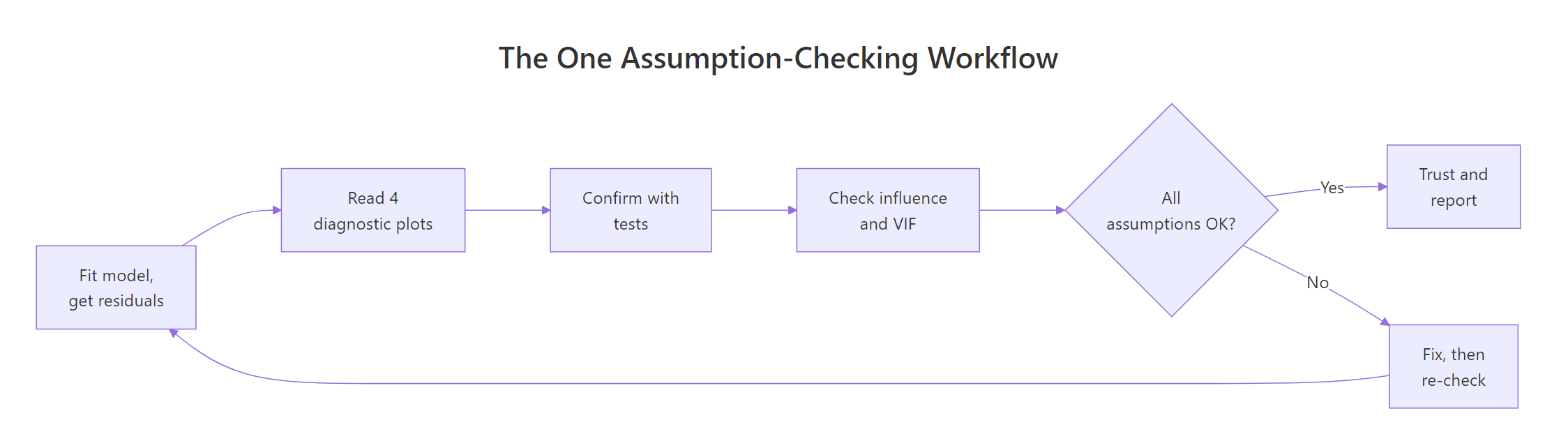
Figure 1: The one workflow. Read the four plots, confirm with tests, check robustness, then fix and re-check.
Running that gives you the four-panel picture below. Each panel maps to one part of the workflow.
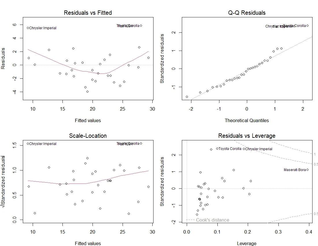
Figure 2: The four base-R diagnostic plots for mpg ~ wt + hp, produced by plot(model).
Here is which panel answers which question. We walk through each one in its own section next.
| Diagnostic plot | Checks | You want to see |
|---|---|---|
| Residuals vs Fitted | Linearity | A flat, patternless band |
| Normal Q-Q | Normality | Points hugging the diagonal |
| Scale-Location | Equal variance | A flat line, even spread |
| Residuals vs Leverage | Influential points | No point far to the right |
Try it: Pull the residuals and fitted values out of the model into your own variables, then look at the first few residuals.
Click to reveal solution
Explanation: residuals() returns one number per row: how far that car's real mpg sits above or below the model's prediction. Every check that follows reads these numbers.
How do you check linearity?
Linearity asks a simple question: is a straight line the right shape for this relationship? If the true pattern curves but you fit a line, the model will over-predict in some regions and under-predict in others, and the residuals will show it.
The tool is the Residuals vs Fitted plot (the top-left panel). You plot each residual against the value the model predicted. If a line is the right shape, the residuals scatter randomly above and below zero with no drift. If the relationship curves, the residuals form a U or an arch.
Run that and look at the red trend line. For our model it dips in the middle and rises at both ends, a gentle bowl shape. That hints the straight line is missing some curvature. A quick numeric check confirms the hunch. The RESET test asks whether adding squared and cubed versions of the fitted values would improve the model; if they would, the plain line is too simple.
The p-value is 0.003, well below 0.05. That is evidence of mild curvature: the relationship between these predictors and mpg bends a little, and a straight line does not fully capture it. This is not a disaster, and we will straighten it out in the fixes section. For now, note it down.
Try it: Run the RESET test on the simpler mpg ~ wt model. Does the one-predictor version also show curvature?
Click to reveal solution
Explanation: The p-value is 0.013, still under 0.05. The mpg-versus-weight curve bends too, which is a well-known feature of fuel-economy data.
How do you check that the residuals have constant variance?
Constant variance, or homoscedasticity, means the residuals are equally spread across the whole range of predictions. The model should be about as accurate for light cars as for heavy ones. When the spread grows as predictions get larger, you get a funnel shape, and that is called heteroscedasticity.
Why care? Heteroscedasticity does not bias your coefficients, but it makes the standard errors wrong, and every p-value and confidence interval the model reports is computed from those standard errors, so they become unreliable too. The picture below shows the two cases side by side so you know what you are looking for.
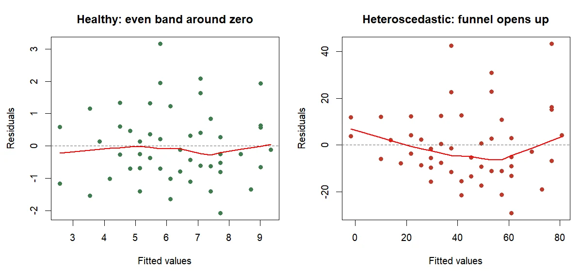
Figure 3: A healthy residual plot (left) versus a heteroscedastic funnel (right).
The Scale-Location plot (bottom-left panel of plot(model)) is built for this. It puts the size of each residual on the y-axis, so a rising trend means the spread is growing.
Eyeballing a plot is a good start, but a formal test removes the guesswork. The Breusch-Pagan test checks whether residual size is related to the fitted values. A small p-value means the variance is not constant.
The p-value is 0.64, far above 0.05, so there is no evidence of a variance problem. Our model passes this check cleanly: the spread of errors is steady across light and heavy cars.
Try it: The cars dataset (stopping distance versus speed) is a classic funnel. Run the Breusch-Pagan test on it and see how the p-value compares.
Click to reveal solution
Explanation: At 0.073 the p-value sits just above 0.05, so the test is borderline. The residual plot for this model shows a clear funnel, which is why plots and tests are best read together.
How do you check that the residuals are normal?
Normality asks whether the residuals follow the familiar bell curve. This matters most for small samples, where the t-tests and confidence intervals lm() reports lean on the normal shape. With large samples the model is forgiving, because averages tend toward normal on their own.
The tool is the Normal Q-Q plot (top-right panel). It sorts your residuals and plots them against the values you would expect from a perfect normal distribution. If the residuals are normal, the points fall along the straight diagonal. Curved-away tails mean skew or heavy outliers.
The matching test is Shapiro-Wilk, which returns a single p-value. A small p-value means the residuals depart from normal.
The p-value is 0.034, just under 0.05, so there is a mild departure from normality. Looking back at the Q-Q plot, only a couple of high-mileage cars at the top pull away from the line. With 32 rows, Shapiro-Wilk is sensitive enough to flag a small wobble, so this is a "keep an eye on it" result, not a red alert.
Try it: Confirm the test behaves by feeding it 100 values you know are normal. Set a seed first so your result matches.
Click to reveal solution
Explanation: The p-value is 0.99, nowhere near significant, which is exactly what you want when the data really is normal. A high p-value is the "no problem here" signal.
How do you check that the residuals are independent?
Independence means one row's error tells you nothing about the next row's error. This assumption is usually fine for a plain sample of unrelated observations, but it breaks for data collected in order, such as measurements over time or along a spatial path, where neighbours tend to be similar.
The standard test is Durbin-Watson, which looks for correlation between each residual and the one before it. Its statistic runs from 0 to 4, and a value near 2 means no autocorrelation. Values near 0 mean strong positive autocorrelation.
The statistic is 1.36 with a p-value of 0.02, which looks like a problem. Here is the judgment call that separates a mechanical check from a real one: mtcars rows are just car models listed in a book, not a time sequence, so "the next row" has no real meaning. A significant Durbin-Watson result on unordered data is an artifact of the arbitrary row order, not a genuine violation. This check only carries weight when your rows have a true order.
Try it: The statistic's distance from 2 measures the size of the autocorrelation. Compute how far our Durbin-Watson value sits from 2.
Click to reveal solution
Explanation: The statistic sits 0.638 below 2. The further below 2, the stronger the positive autocorrelation would be, if the row order were meaningful here.
How do you find influential outliers?
Not every unusual point matters. A point is influential only when it both sits far from the others in predictor space (high leverage) and has a large residual. Such a point can single-handedly tilt the fitted line toward itself, so the whole model bends to accommodate one observation.
The Residuals vs Leverage plot (bottom-right panel) shows leverage on the x-axis, so influential points appear in the far right. The one-number summary is Cook's distance, which combines leverage and residual size into a single score per row.
A common rule of thumb flags any row whose Cook's distance is above 4 / n, where n is the number of rows. Let's list the cars that clear that bar.
Four cars clear the threshold, with the Chrysler Imperial the most influential at 0.424. Flagging a point is not the same as deleting it. The right move is to investigate: is it a data-entry error, or a genuine but unusual car? We test its actual impact in the fixes section by refitting without it.
Try it: Find the single most influential car by name using which.max() on the Cook's distances.
Click to reveal solution
Explanation: which.max() finds the position of the biggest Cook's distance, and names() turns that position back into the car's name.
How do you check for multicollinearity between predictors?
The last check is the one that is about the predictors rather than the residuals. Multicollinearity happens when two or more predictors carry nearly the same information. When weight and horsepower move together, the model cannot tell whose effect is whose, so the coefficients become unstable and their standard errors balloon.
The measure is the Variance Inflation Factor (VIF). For each predictor, you regress it on all the other predictors and read off that helper model's R-squared. The formula turns that into an inflation factor:
$$\text{VIF}_j = \frac{1}{1 - R_j^2}$$
A VIF of 1 means the predictor shares nothing with the others; a common rule of thumb treats anything above 5 as worth investigating and above 10 as a real problem. You can compute it directly in base R with a short helper.
Both predictors sit at 1.77, comfortably below 5. Weight and horsepower are correlated, but not so tightly that the model struggles to separate them. In everyday work you would reach for the car package's one-liner instead of the helper above. Run this in your local R session, since car is not part of the in-browser toolkit:
library(car)
round(vif(model), 3)
#>    wt    hp
#> 1.767 1.767performance::check_model(model) produces an annotated panel of all the checks in this guide, which is handy once you know how to read each one on its own.Try it: Add disp (engine displacement) as a third predictor and recompute the VIFs. Displacement is closely tied to weight, so watch what happens.
Click to reveal solution
Explanation: Displacement's own VIF is 7.3, and adding it raises weight's VIF to 4.8, because engine size and weight measure overlapping things. This is when you would consider dropping one of the two.
What should you do when an assumption is violated?
Our workflow flagged two real issues on mpg ~ wt + hp: mild curvature (the RESET test) and slightly non-normal residuals (Shapiro-Wilk). Here are the three moves that fix the large majority of problems, starting with the one that fixes ours.
Move 1: transform the response. When the relationship curves or the residuals are skewed, modelling the response on a log scale often straightens everything at once. Let's refit with log(mpg) and re-run the two checks that failed.
Both p-values jumped above 0.05: RESET went from 0.003 to 0.31, and Shapiro-Wilk from 0.034 to 0.27. The curvature and the skew are gone. Better still, the fit improved rather than suffered.
Adjusted R-squared rose from 0.815 to 0.860. One small change to the response scale repaired both violations and told a cleaner story about the data.
Move 2: use robust standard errors. Sometimes you cannot or do not want to transform, yet the variance is not constant. You can keep the model and just correct the standard errors so the p-values stay honest. The sandwich package supplies heteroscedasticity-consistent errors that coeftest() reads. To see it work, here is a dataset built with strong, deliberate heteroscedasticity.
Now recompute the same model with robust standard errors and compare.
The estimate for x is identical at 3.13; only its standard error changed, from 0.83 up to 1.09. The naive version was overstating the model's certainty. Robust errors leave the coefficients alone and just report the wider, more honest uncertainty.
Move 3: investigate influential points, do not just delete them. Our Cook's distance check flagged the Chrysler Imperial. The honest test is to refit without it and see whether the conclusions actually move.
The weight coefficient shifts from -3.88 to -4.42 when the car is removed. That is a noticeable nudge, but the story is unchanged: weight still has a strong, negative, significant effect. Since the point does not flip any conclusion and is a real car, you keep it and note its influence.
The whole workflow in one function
Once you have done this a few times, package it so you never have to remember the order again. This small function runs every check and returns a tidy table of p-values plus the influence count and worst VIF.
For the four test rows, a value below 0.05 is a flag worth reading a plot about; the last two rows are counts, not p-values. Run check_assumptions(logmod) and you will see the first three flags clear.
Practice Exercises
These combine several checks from the guide. Use the distinct variable names shown so your work does not overwrite the tutorial's model.
Exercise 1: Run the workflow on a new model
Fit a model of stopping distance on speed with lm(dist ~ speed, data = cars), then run the four core checks (RESET, Breusch-Pagan, Shapiro-Wilk, Durbin-Watson) and read off which assumption is most clearly violated.
Click to reveal solution
Explanation: Normality is the clearest violation at 0.0215, with variance close behind at 0.073. Linearity and independence are fine. The next exercise fixes it.
Exercise 2: Fix the cars model with a transform
The stopping-distance model has non-normal, funnel-shaped residuals. Physics suggests distance grows with the square of speed, so a square-root transform of dist is a natural fix. Refit as sqrt(dist) ~ speed and re-run the two checks that were weakest.
Click to reveal solution
Explanation: Both p-values leap upward, Breusch-Pagan to 0.92 and Shapiro-Wilk to 0.31. The square-root scale flattened the funnel and normalised the residuals in one move.
Exercise 3: Write a pass/fail helper
Write a function all_ok(m) that returns TRUE only when the RESET, Breusch-Pagan, and Shapiro-Wilk tests all have p-values above 0.05. Test it on the original model and on logmod from the fixes section.
Click to reveal solution
Explanation: The raw model fails because linearity and normality were flagged; the log model passes all three. This is the same conclusion the fixes section reached, now automated.
Frequently Asked Questions
Which assumption matters most?
Constant variance and linearity usually matter most, because they directly bend your coefficients or corrupt your standard errors. Independence matters intensely but only for ordered data. Normality is the most forgiving, especially once you have a few dozen rows.
Do I really need both the plots and the tests?
Yes, they cover each other's blind spots. Tests give an objective p-value but can flag trivial departures in large samples or miss real ones in small samples. Plots show the shape and severity a p-value hides. Read them together, as the cars example showed, where a borderline test sat next to an obvious funnel.
My Shapiro-Wilk test is significant. Is my model ruined?
Probably not. On 30 or more rows the test is sensitive to tiny wobbles, and linear regression is robust to mild non-normality. Look at the Q-Q plot: if only a couple of points stray at the tails, you are usually fine. Worry when the whole pattern curves away from the line.
What counts as a "good enough" VIF?
A VIF of 1 is ideal. Below 5 is generally comfortable. Between 5 and 10 is a yellow flag worth a second look, and above 10 signals serious multicollinearity where you should drop or combine predictors.
Can I check assumptions before fitting the model?
No, and that is the key idea of this guide. Three of the four assumptions are about the model's residuals, which only exist after you fit. Fit first, then diagnose, then fix and refit if needed.
Summary
Checking model assumptions is one short loop you run on every linear model: read the four diagnostic plots, confirm with a quick test, scan for influential points and collinearity, then fix and re-check anything that fails.
| Assumption | Diagnostic plot | Confirming test | Passes when | If it fails |
|---|---|---|---|---|
| Linearity | Residuals vs Fitted | RESET (resettest) |
p > 0.05, flat band | Transform or add a term |
| Equal variance | Scale-Location | Breusch-Pagan (bptest) |
p > 0.05, even spread | Transform or robust errors |
| Normality | Normal Q-Q | Shapiro-Wilk (shapiro.test) |
p > 0.05, points on line | Transform, or ignore if mild |
| Independence | Residual order | Durbin-Watson (dwtest) |
statistic near 2 | Use a time-series model |
| No influential points | Residuals vs Leverage | Cook's distance | none above 4/n | Investigate, rarely remove |
| No multicollinearity | (none) | VIF | below 5 | Drop or combine predictors |
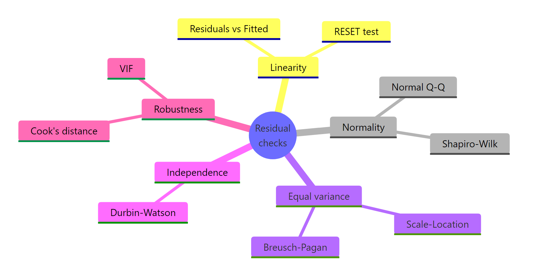
Figure 4: Each assumption, its diagnostic plot, and its confirming test.
The habit to build is simple. Fit the model, glance at plot(model), confirm the two or three checks that matter for your data, and only trust the p-values once the residuals have earned it.
References
- Zeileis, A. and Hothorn, T. lmtest package (Breusch-Pagan, Durbin-Watson, RESET). CRAN. Link
- Zeileis, A. sandwich package (heteroscedasticity-consistent covariance). CRAN. Link
- James, G., Witten, D., Hastie, T., and Tibshirani, R. An Introduction to Statistical Learning, chapter 3 on potential problems in regression. Link
- R Core Team. plot.lm reference: the four diagnostic plots. Link
- R Core Team. shapiro.test reference. Link
- NIST/SEMATECH e-Handbook of Statistical Methods: examining residuals. Link
- Robinson, D. broom vignette: tidying model output with
tidy()andglance(). Link
Continue Learning
- Linear Regression in R: fit and interpret the model this guide diagnoses.
- Assumptions of Linear Regression: a deeper reference that walks through every classical assumption in turn.
- Outlier Treatment With R: what to do once Cook's distance flags an influential point.