Crossed vs Nested Random Effects in R
Nested and crossed random effects describe two ways grouping factors can relate in a mixed model. Nested means each inner level sits inside exactly one outer level, like classes within schools. Crossed means the two factors overlap, like people who each answer every question. This guide builds both ideas from scratch on small datasets, shows the exact lme4 formula for each, and walks you through the one mistake that quietly wrecks a nested model. It uses base R plus lme4, and every example runs right here in your browser.
What is the difference between crossed and nested random effects?
Real data almost never arrives as a flat list of independent rows. It comes in groups: pupils in classrooms, measurements from casks, ratings from people. A mixed model handles data like this by estimating how much the outcome shifts from one group to the next, and that group-to-group variation is what we call a random effect. Sometimes one grouping sits inside another, forming a hierarchy. Sometimes two groupings sit side by side and overlap. Getting that structure right matters, because the wrong choice silently changes your variance estimates. Let's make both structures concrete on a small, real dataset.
We will start with Pastes, a dataset that ships with lme4. It records the strength of an industrial paste, delivered in batches, with a few casks sampled from each batch, and two strength tests per cask.
Each row is one strength test. batch is the delivery batch (labelled A to J), cask is which cask within that batch (labelled a, b, c), and sample is a combined label like A:a that names one physical cask. Notice the first six rows are all batch A, with casks a, b, and c. Let's count the levels to see the shape of the data.
So there are 10 batches, 3 casks in each, which makes 30 physical casks, and 60 rows because each cask was tested twice. Here is the subtle part. The cask labels a, b, and c are reused in every batch, but cask "a" in batch A is a completely different physical cask from cask "a" in batch B. Each cask belongs to one and only one batch. That is nesting: the inner level (cask) lives inside exactly one outer level (batch).
Crossing is the opposite picture. Imagine 20 people who each rate the same 5 films. Every person meets every film, so the "person" grouping and the "film" grouping overlap completely. Film 1 is the same film for all 20 raters. Neither factor sits inside the other; they cross.
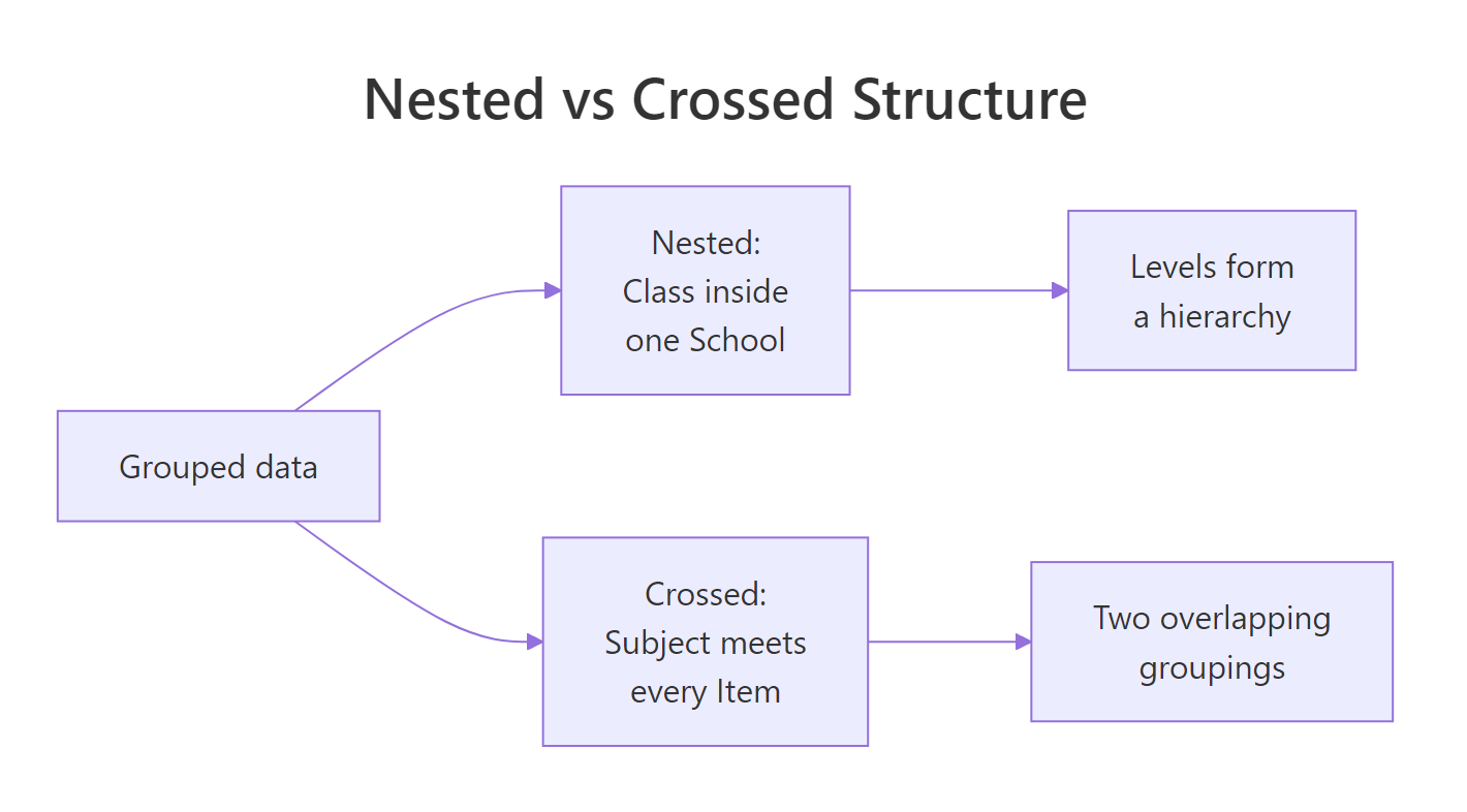
Figure 1: Nested groupings form a hierarchy; crossed groupings overlap.
Try it: Confirm the nesting by counting how many distinct casks each batch actually contains. The helper tapply() runs a function within each batch, and nlevels(droplevels(x)) counts the casks that are truly present.
Click to reveal solution
Explanation: Every batch contains exactly 3 casks. Because those casks are different physical objects in each batch, cask is nested within batch, giving 10 times 3 equals 30 distinct casks in total.
How do you fit a nested random effects model?
To fit a nested model you use lmer(), the main function for fitting mixed models in lme4. There is no fixed predictor here, just the overall average, so the formula is strength ~ 1, where the 1 stands for that single intercept. The random part goes in parentheses, and the bar | means "grouped by" the factor on its right. For nesting, lme4 gives you a shortcut: write (1 | batch/cask), which reads as "a per-group intercept for cask nested within batch". Let's fit it and read the output.
The "Random effects" block is where the structure shows up, and it has three rows. The cask:batch row is the variation from one cask to another within a batch, with a standard deviation of about 2.9. The batch row is the variation from one whole batch to another, with a standard deviation of about 1.3. The Residual row is the leftover test-to-test noise inside a single cask, at about 0.8. The single fixed effect, the intercept of 60.05, is just the overall average paste strength.
Reading those three numbers is the payoff. Most of the variation lives at the cask level, not the batch level, which tells you that casks within a batch differ more than batches differ from each other. That is a real, actionable finding about where the inconsistency in this paste comes from.
lme4 being precise: it built a fresh grouping that respects the nesting, rather than pooling the three cask letters.The slash is only a shortcut. Under the hood, (1 | batch/cask) expands into two separate terms: one for the batch and one for the cask-within-batch combination. Writing those two terms out by hand gives an identical fit.
The variances match the previous fit to the last decimal. The term (1 | batch:cask) builds a random effect for each unique batch-and-cask combination, which is precisely the nesting. So (1 | batch/cask) and (1 | batch) + (1 | batch:cask) are two spellings of the same model.
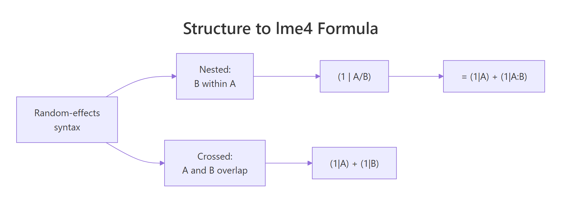
Figure 2: How each structure maps to an lme4 random-effects formula.
Try it: The VarCorr() output is nice to read but hard to compute with. Turn it into a plain data frame with as.data.frame() and print the group, variance, and standard-deviation columns.
Click to reveal solution
Explanation: The vcov column is the variance and sdcor is the standard deviation. Having them as a data frame lets you do arithmetic on them, which we will use later to compute variance shares.
How do you fit crossed random effects?
Now let's switch to a genuinely crossed design. The clearest way to see crossing is to build it, so we will simulate a small study where 24 people each rate 12 items, and every person rates every item exactly once. Each score is the sum of a person effect, an item effect, and some noise. We fix the random seed so you get the same numbers every time.
Each row is one person responding to one item. The expand.grid() call creates every subject-and-item combination, and the score is built from a subject shift plus an item shift plus random noise. Now let's confirm the crossing by tabulating subjects against items.
Every cell is 1, meaning each subject appears with each item. And crucially, item I01 is the same physical item shown to all 24 subjects, unlike cask "a" which was a different cask in every batch. That shared identity is what makes subjects and items truly crossed. You fit crossed random effects with two separate bar terms, one per factor.
There are now two grouping rows sitting side by side, subject and item, plus the residual. Neither is nested in the other. The subject standard deviation of 22.5 says people differ from each other by that much on average, and the item standard deviation of 16.5 says items differ by a bit less. The model estimated both, at the same time, from the same data. Let's confirm how many groups sit on each side.
There are 24 subject groups and 12 item groups, exactly the design we built. Compare that to the nested Pastes model, where the inner group count was 30, equal to 10 batches times 3 casks. In a crossed design the two counts are independent; in a nested design the inner count is the outer count multiplied through.
Try it: Read the two variance components as standard deviations to decide which side varies more. Pull the tidy VarCorr() frame and print its group and sdcor columns.
Click to reveal solution
Explanation: Subjects vary more than items, with standard deviations of 22.5 against 16.5. The residual of 26.0 is the noise left after accounting for both the person and the item.
If you like seeing the models written out, here is the contrast in symbols. For the nested paste strength $y$ of cask $j$ inside batch $i$ on test $k$, and for the crossed rating $y$ by subject $s$ of item $t$:
$$y_{ijk} = \beta_0 + b_i + b_{ij} + \epsilon_{ijk} \qquad\qquad y_{st} = \beta_0 + a_s + c_t + \epsilon_{st}$$
Where:
- $\beta_0$ = the overall average, shared by both models
- $b_i$ and $b_{ij}$ = the batch shift and the cask-within-batch shift; the shared index $i$ is the hierarchy
- $a_s$ and $c_t$ = the subject shift and the item shift; the separate indices $s$ and $t$ are the crossing
- $\epsilon$ = the leftover noise
If formulas are not your thing, skip past the equation; the two model fits above already gave you the same information. The one thing worth noticing is the indices: nested effects share an index and stack, while crossed effects use independent indices and overlap.
How can you tell crossed and nested apart?
Here is the trap that catches almost everyone. The lme4 package does not have a separate engine for nested and crossed models. It reads the structure straight from your factor labels. So if the labels are reused, like the casks a, b, c that repeat in every batch, and you write the crossed formula, lme4 will believe there are only three casks in the entire dataset. Let's watch it go wrong.
Compare this to the correct nested fit. The cask standard deviation collapsed from 2.90 down to 0.39, and the residual jumped from 0.82 up to 2.70. The real cask-to-cask variation did not disappear: because the wrong formula pooled the casks into just three groups, the differences between casks in the same batch had nowhere to go and were absorbed into the residual instead. Counting the groups shows exactly what happened.
The model found only 3 cask groups instead of 30. It treated the three labels a, b, and c as if cask "a" were a single cask crossed with all ten batches. That is the implicit-nesting trap, and it silently gives you wrong variance estimates with no error message.
(1 | outer) + (1 | inner) collapses all the inner levels into a handful of label groups. Always check ngrps() against the number of distinct inner units you expect.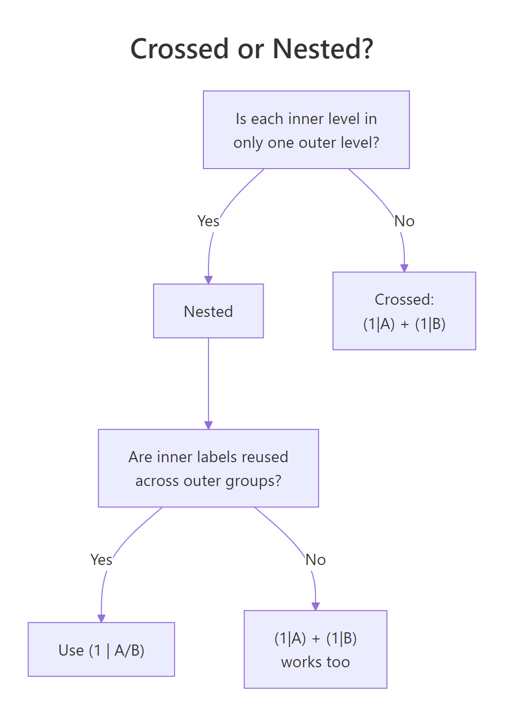
Figure 3: A quick test for whether your factors are crossed or nested.
There are two clean fixes. The first is the slash notation you already know, (1 | batch/cask), which builds the correct groups for you. The second is to give the inner units unique labels so the plain crossed formula works. The Pastes data already includes such a column, sample, which holds labels like A:a and B:a that never repeat.
These variances are identical to the nested fit from earlier. With unique labels, the plain crossed formula (1 | batch) + (1 | sample) recovers the exact nested model, because there are now 30 distinct sample labels for the 30 physical casks. Let's look at those labels.
Each label pastes the batch onto the cask, so A:a and B:a are recognised as different casks. This is what people mean when they say nesting is handled "for free" as long as your labels are unique.
lme4 engine is identical either way. Your only job is to make sure the factor labels tell the truth: either use the slash notation, or give inner units globally unique labels. Once the labels are right, the same lmer() call fits nested, crossed, or any mix of the two.Try it: Build unique cask labels yourself with interaction(), which pastes two factors together, then count how many distinct labels you get.
Click to reveal solution
Explanation: You get 30 unique labels, one per physical cask. Now (1 | batch) + (1 | cask_id) would fit the correct nested model, because cask_id never repeats across batches.
What if not every combination appears?
Real crossed data is often incomplete. Maybe not every person had time to rate every item, so some subject-and-item combinations are missing. This is called partially crossed data, and the good news is that lme4 handles it with no special syntax at all. You still write (1 | subject) + (1 | item). Let's prove it by randomly dropping 48 of the 288 responses.
The variance components barely moved from the fully crossed fit, even though we threw away a sixth of the data. The same formula still works. We can confirm that some subject-and-item cells really are empty now.
The TRUE tells us at least one combination is missing, so the design is no longer fully crossed. Yet lmer() fit the model with the same two-term formula and no special handling. Partially crossed data is the normal case in fields like psychology and linguistics, and it needs nothing beyond the two-bar-term formula.
InstEval dataset that ships with lme4 holds over 73,000 university course ratings, crossing thousands of students with hundreds of instructors, most of whom never met. The very same (1 | student) + (1 | instructor) syntax fits it. Partial crossing is expected, not a problem.Try it: Confirm exactly how many responses survived the drop by comparing the row counts of the full and partial datasets.
Click to reveal solution
Explanation: We kept 240 of the original 288 responses, dropping 48. The model still estimated stable subject and item variances from what remained.
Practice Exercises
These exercises pull together the ideas above. Try each one before opening the solution. They use their own variable names, prefixed with my_, so they will not disturb the models you fit earlier in the page.
Exercise 1: What share of variance sits at each level?
Fit the nested Pastes model, then compute what fraction of the total random variance sits at each level: cask-within-batch, batch, and residual. Turning VarCorr() into a data frame makes the arithmetic easy.
Click to reveal solution
Explanation: About 78 percent of the random variation is cask-to-cask within a batch, only 15 percent is between batches, and a mere 6 percent is test-to-test noise. The casks are the main source of inconsistency in this paste.
Exercise 2: Turn the crossed variances into percentages
Using the crossed_df data from the crossed section, fit the crossed model and report each source of variation as a percentage of the total. This is a common way to summarise where the variability in ratings comes from.
Click to reveal solution
Explanation: Subjects account for 35 percent of the variance and items for 19 percent, while 47 percent is residual noise. Because the two grouping factors are crossed, you can read their contributions as two separate slices of the same pie.
Exercise 3: Fix a dataset with reused labels
Build a small schools-and-classes dataset where class labels C1 to C4 repeat across six schools. Then show that the naive crossed formula finds only 4 class groups, while the correct nested formula finds all 24. This is the implicit-nesting trap in miniature.
Click to reveal solution
Explanation: The naive crossed formula collapses the 24 real classes into just 4 label groups, because class C1 appears in every school. The nested formula, or equivalently unique labels, recovers all 24 classes. Always let ngrps() catch this before you trust a fit.
Frequently Asked Questions
What is the difference between crossed and nested random effects in one sentence?
Nested means each level of the inner factor belongs to exactly one level of the outer factor, forming a hierarchy like casks within batches, so you write (1 | outer/inner). Crossed means each level of one factor appears with every level of the other, like subjects who each rate every item, so you write (1 | factor1) + (1 | factor2). The engine is the same; only the formula and the data structure differ.
Is the crossed-or-nested distinction about the data or the model?
It is about the data. lme4 uses identical computation for both, and it decides the structure entirely from your factor labels. Your responsibility is to describe the data honestly: use the slash notation when inner labels repeat across outer groups, or give every inner unit a globally unique label. Get the labels right and the same lmer() call handles any structure.
Why did my inner variance collapse to nearly zero?
That is the classic sign of the implicit-nesting trap. You wrote a crossed formula like (1 | school) + (1 | class), but your class labels are reused across schools, so lme4 pooled them into a few label groups and pushed the real class variation into the residual. Check with ngrps(): if it reports far fewer inner groups than you have real inner units, switch to (1 | school/class) or build unique labels with interaction().
When should I use (1 | a/b) versus (1 | a) + (1 | b)?
Use (1 | a/b) when b is nested in a, meaning each level of b sits inside one level of a. Use (1 | a) + (1 | b) when a and b are crossed, meaning they overlap. The one situation that trips people up is nested data with reused inner labels: there, (1 | a) + (1 | b) is wrong, and you need either the slash or unique labels. When inner labels are already unique, the two spellings give the same fit.
Can a model have both crossed and nested random effects?
Yes, and it is common. You might have students crossed with items, while students are also nested within schools. You simply combine the terms, for example (1 | school/student) + (1 | item). Each term describes one piece of the structure, and lme4 fits them together. The same rules apply to every term: nesting uses a slash or unique labels, crossing uses separate bar terms.
Summary
Nested and crossed random effects are two ways grouping factors relate, and choosing correctly is the difference between right and wrong variance estimates. Nested factors form a hierarchy and use a slash; crossed factors overlap and use two separate bar terms. The one trap to remember is that lme4 reads structure from labels, so reused inner labels must be fixed with the slash or with interaction().
| Formula piece | Structure it describes | When to use it | ||
|---|---|---|---|---|
| `(1 \ | a/b)` | b nested in a (hierarchy) | Each inner level sits in one outer level | |
| `(1 \ | a) + (1 \ | a:b)` | Same nesting, written out | When you want the two rungs explicit |
| `(1 \ | a) + (1 \ | b)` | a and b crossed (overlap) | Both factors classify every response |
interaction(a, b) |
Unique inner labels | Nested data whose inner labels repeat |
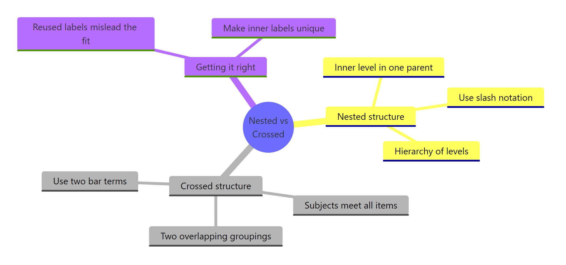
Figure 4: Crossed versus nested random effects at a glance.
The biggest ideas to carry with you: nested means inside and crossed means overlapping, the slash (1 | a/b) is just shorthand for two terms, and whenever an inner variance looks suspiciously small, check ngrps() for the implicit-nesting trap.
References
- Bates, D., Mächler, M., Bolker, B., & Walker, S. (2015). Fitting Linear Mixed-Effects Models Using lme4. Journal of Statistical Software, 67(1). Link - the canonical paper behind
lme4, covering crossed and nested random effects. - Bates, D. lme4: Models With Multiple Random-effects Terms, Chapter 2. Link - the source of the
Pastesexample and the definitive treatment of nested versus crossed. - lme4 package vignette: Fitting Linear Mixed-Effects Models Using lme4. Link - the official walkthrough of
lmer()syntax. - Bolker, B. GLMM FAQ. Link - practical answers on implicit nesting, crossed effects, and when labels need to be unique.
- Vanderhaeghe, F. Nested and crossed random effects in lme4. Link - a clear, example-driven explanation of the same distinction.
- Gelman, A., & Hill, J. (2007). Data Analysis Using Regression and Multilevel/Hierarchical Models. Cambridge University Press. Link - the standard textbook on multilevel structure and grouping.
Continue Learning
- Random Intercepts and Slopes with lme4 in R - the companion guide that explains what a random intercept and slope are, and how partial pooling works.
- Multilevel Models in R - a broader look at hierarchical models, the setting where nested random effects appear most often.
- How to Read lm() Output in R - the fixed-effects half of any mixed model is ordinary regression, and this covers how to read it.