How to Read lm() Output in R Line by Line
When you fit a model with lm() and call summary() on it, R prints a wall of numbers that can look like a foreign language. This guide reads that output one line at a time, so by the end you can glance at any regression summary and know exactly what each value means and which ones you can trust. Everything here uses base R, no extra packages.
Where should you look first in lm() output?
The first time you see a regression summary, it feels like too much at once. The trick is to stop reading it as one block and start seeing it as four stacked sections, each answering a different question. Let's fit a real model and print it so we have something concrete to point at.
We will predict a car's fuel economy (mpg, miles per gallon) from its weight (wt, in thousands of pounds) using the built-in mtcars data. Heavier cars burn more fuel, so we expect weight to pull mileage down.
That is the whole printout. Press Run and it appears in your browser in a second. Now look at its shape rather than its numbers: there are four labelled areas separated by blank lines.
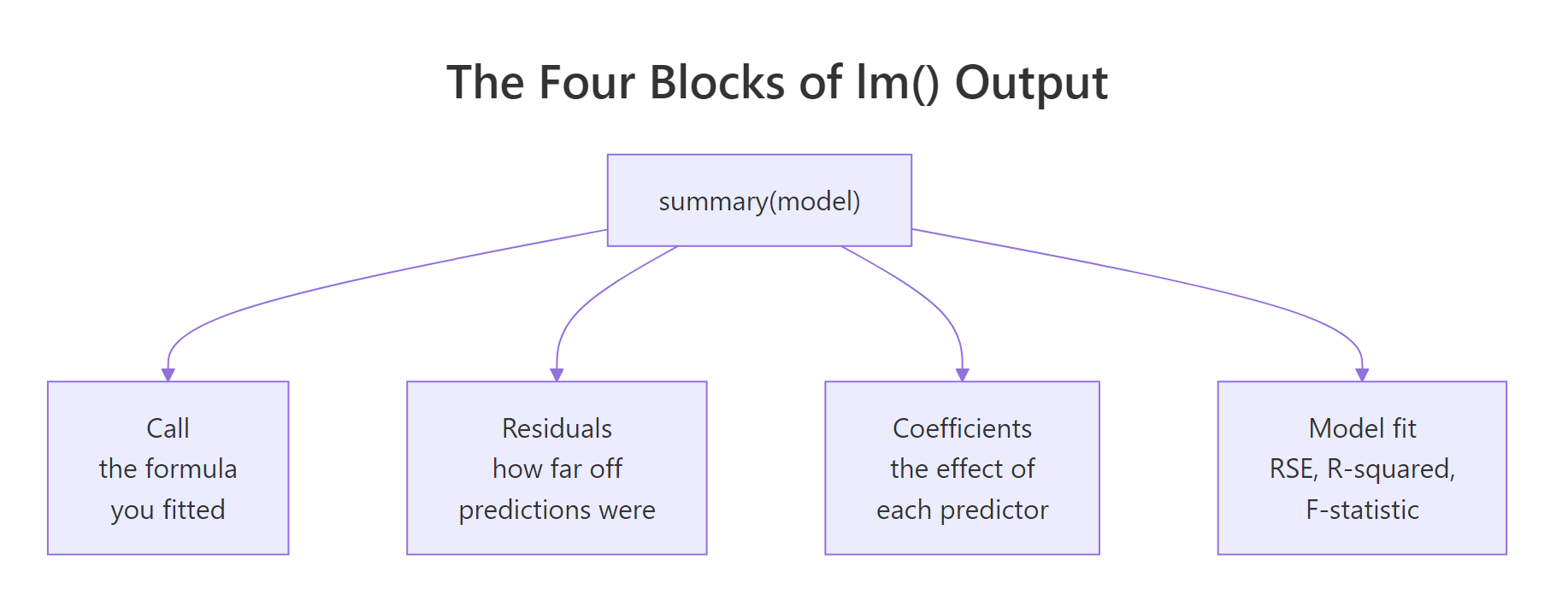
Figure 1: The four stacked blocks of summary() output on an lm model.
Here is what each block is for, reading top to bottom:
- Call repeats the formula you fitted, so you can confirm R modelled what you meant.
- Residuals summarise how far the predictions missed the actual values.
- Coefficients is the heart of the output: the effect of each predictor, with a measure of how sure we are.
- Model fit (the last three lines) tells you how good the model is overall.
We will walk through all four in that order. The rest of this guide is basically a magnified tour of this one printout.
summary() output stops feeling intimidating.Try it: Fit a model that predicts mpg from horsepower (hp) instead of weight, then pull out just its Multiple R-squared value.
Click to reveal solution
Explanation: summary() returns an object, and $r.squared pulls the R-squared straight out of it. Horsepower alone explains about 60 percent of the variation in mileage, a bit less than weight did.
What is the Call line telling you?
The top block is the easiest to read and the easiest to skip, which is a mistake. The Call line simply echoes the formula and data you gave to lm(). Its job is to let you confirm, at a glance, that R fitted the model you intended.
Let's pull the Call out on its own so you see it clearly.
This says the response is mpg, the single predictor is wt, and the data came from mtcars. The tilde ~ reads as "is modelled by", so mpg ~ wt means "mpg is modelled by wt".
Why does this matter? Because it is your receipt. If you meant to control for horsepower and the Call shows only wt, you caught the mistake before drawing any conclusions. If you filtered your data first, the Call reminds you which version of the data went in.
Try it: Fit a model of mpg on horsepower and read back its Call line to confirm the formula.
Click to reveal solution
Explanation: The Call confirms the predictor is hp, not wt. Checking this one line prevents you from mixing up two similar models.
How do you read the Residuals summary?
Before we judge the model, we need to know how badly it misses. A residual is the gap between what actually happened and what the model predicted: actual value minus predicted value. A car whose real mileage is 21 when the model guessed 19 has a residual of +2.
R does not print all 32 residuals. Instead it gives you a five-number summary: the smallest residual, the first quartile (the value a quarter of the residuals fall below), the median, the third quartile (three quarters fall below it), and the largest. Let's reproduce exactly those five numbers.
Match these against the Residuals: line in the full summary above: Min is the 0 percent value (-4.543), Median is the 50 percent value (-0.125), and Max is the 100 percent value (6.873). They are the same numbers, just relabelled.
What are you checking for here? Two quick things. First, the median should sit close to zero, which means the model is not systematically guessing too high or too low. Ours is -0.125, comfortably near zero. Second, the smallest and largest residuals should be roughly balanced in size. Here the biggest miss is +6.87 (one car did much better than predicted) against -4.54 on the low side, a mild right lean but nothing alarming.
Try it: Find the single largest positive residual (the car that beat its prediction by the most) and which car it is.
Click to reveal solution
Explanation: The Fiat 128 got about 6.87 more miles per gallon than a weight-only model expected. Large residuals like this flag cars the model does not explain well, often a hint that another predictor is missing.
How do you read the Coefficients table row by row?
This block holds the actual model estimates, so we will slow down. The Coefficients table has one row per term (the intercept plus each predictor) and four columns. Let's print just the table as raw numbers so nothing is hidden.
Read it one column at a time.
The Estimate column is the number you came for. For the wt row it is -5.34. Because weight is measured in thousands of pounds, this means: for every extra 1,000 pounds of weight, the model expects mileage to drop by about 5.34 miles per gallon. The sign matters as much as the size. Negative confirms our intuition that heavier cars go fewer miles per gallon.
The (Intercept) row is the predicted mpg when every predictor is zero, so here it is the predicted mileage of a car that weighs zero pounds: 37.29. A weightless car is impossible, so treat the intercept as the anchor point of the line rather than a real forecast. It positions the line; it is not a prediction you would ever use.
The Std. Error column measures how much the estimate would move if you collected the data again. A small standard error means the estimate is pinned down tightly. The slope estimate of -5.34 has a standard error of only 0.56, small next to the estimate itself, so weight's effect is measured precisely rather than being a vague guess.
The t value column combines the two columns before it. It asks a simple question: how big is the estimate compared to its own uncertainty? You get it by dividing the Estimate by the Std. Error.
$$t = \frac{\hat{\beta}}{SE(\hat{\beta})}$$
Where:
- \\(\hat{\beta}\\) is the estimated coefficient (the Estimate column).
- \\(SE(\hat{\beta})\\) is its standard error (the Std. Error column).
Let's confirm the t value for wt is really just that division.
That -9.56 matches the t value column exactly. A t value of -9.56 means the slope sits more than nine standard errors below zero, which is very far from "no effect". The last column, Pr(>|t|), turns that distance into a probability, and we tackle it in the next section.
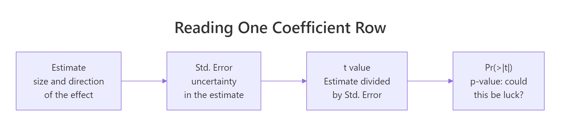
Figure 2: How to read a single coefficient row from left to right.
Try it: Use the intercept and slope to predict the mileage of a car weighing 3,500 pounds (so wt = 3.5).
Click to reveal solution
Explanation: Plugging the weight into intercept + slope * weight gives about 18.6 mpg. This is exactly what the regression line does for any weight you feed it. unname() just drops the leftover label so you see a clean number.
What do the significance stars and codes mean?
The last column of the table, Pr(>|t|), is the p-value. It answers a cautious question: if this predictor truly had no effect, how often would random sampling alone hand us an estimate this large? A small p-value means "almost never by luck", which is your evidence that the effect is real.
Let's read the two p-values on their own.
Both are tiny. The wt p-value of 1.29e-10 is 0.000000000129, so weight almost certainly has a real link to mileage. R also refuses to print a p-value below its precision floor, so anything smaller shows as < 2e-16, which is why the intercept reads < 2e-16 in the top printout even though its exact value here is about 8e-19. In the full printout R rounds these and adds a star key so you do not have to squint at exponents. Those are the significance codes:
***means the p-value is below 0.001 (strongest evidence).**means below 0.01.*means below 0.05, the usual cutoff for "statistically significant"..means below 0.10 (borderline).- a blank means above 0.10 (no real evidence).
Both rows earned ***, so both are strongly supported by the data.
Try it: Check directly whether the wt p-value clears the strongest bar, below 0.001.
Click to reveal solution
Explanation: TRUE confirms the p-value is under 0.001, which is why R printed three stars next to wt.
What do the last three lines mean (RSE, R-squared, F-statistic)?
The bottom three lines grade the model as a whole rather than one predictor at a time. Let's pull each number out so we can label it precisely.
Here is what each one tells you.
The Residual standard error (3.05, printed as s$sigma) is the typical size of a prediction miss, in the same units as the response. So a weight-only model is off by roughly 3 miles per gallon on an average car. The "30 degrees of freedom" beside it is the sample size minus the number of things we estimated (32 cars minus 2 coefficients).
The Multiple R-squared (0.7528) is the share of the variation in mileage that the model explains, on a 0 to 1 scale. About 75 percent of why cars differ in mileage is captured by weight alone. The formula behind it compares the errors your model still makes to the errors you would make with no predictor at all.
$$R^2 = 1 - \frac{\sum_{i}(y_i - \hat{y}_i)^2}{\sum_{i}(y_i - \bar{y})^2}$$
Where:
- \\(y_i\\) is the actual value for car \\(i\\).
- \\(\hat{y}_i\\) is the model's prediction for that car.
- \\(\bar{y}\\) is the average mileage across all cars.
If you are not interested in the formula, skip it. The plain-English version is enough: R-squared is the fraction of the ups and downs in the outcome that the model accounts for.
The Adjusted R-squared (0.7446) is Multiple R-squared with a penalty for the number of predictors. It only rises when a new predictor pulls its weight, which is why it is the fairer number for comparing models of different sizes.
The F-statistic (91.38) and its p-value test the whole model at once: is this model better than one with no predictors at all? A large F with a tiny p-value (1.29e-10 here) says yes. For a model with a single predictor, the F-statistic is just the t value squared, which we can check.
That 91.38 is exactly the F-statistic. The single-predictor F-test and the slope's t-test are the same test seen from two angles.
Try it: Express the residual standard error as a fraction of the average mileage, so you can judge whether a 3 mpg miss is large.
Click to reveal solution
Explanation: The typical miss is about 15 percent of average mileage. Scaling the error against the mean turns an abstract 3.05 into something you can actually reason about.
How does the output change with more than one predictor?
Real models almost always use several predictors. The good news is that the output keeps the same four-block shape; it just grows an extra row in the Coefficients table for each predictor. Let's add horsepower to the weight model and read the changes.
There is now an hp row. Its estimate is -0.032, meaning each extra unit of horsepower is linked to about 0.03 fewer miles per gallon, and its two stars say that link is well supported. With one more predictor in the mix, the way you read each slope changes slightly: every coefficient is now the effect of its predictor while holding the other predictors fixed. So -3.88 for weight is the mileage drop per 1,000 pounds among cars of the same horsepower.
Notice the weight slope shrank from -5.34 to -3.88. That is not an error. Heavier cars tend to have more horsepower, so in the simple model the weight coefficient absorbed part of horsepower's effect too. Separating the two predictors gives each its own share.
The model-fit lines improved: Residual standard error fell from 3.05 to 2.59, and Adjusted R-squared rose from 0.745 to 0.815. Let's compare the two adjusted values side by side.
Adding horsepower genuinely helped: the adjusted score went up, so the extra predictor earned its place.
Try it: Add cylinders (cyl) as a third predictor and see whether Adjusted R-squared keeps climbing.
Click to reveal solution
Explanation: Adjusted R-squared inched up from 0.815 to 0.826, so cylinders add a little, though far less than horsepower did. A tiny gain like this is a judgment call, not an automatic keep.
How do you go beyond summary(): confidence intervals and predictions?
The summary shows single best-guess numbers, but a good analyst also wants the range around them and a way to forecast new cases. Two base R functions handle this, and both read straight off the model you already fitted.
First, confint() turns each Estimate into a plausible range, called a confidence interval. It is the interval within which the true coefficient most plausibly sits.
Read the wt row as: the true weight effect is most plausibly between -5.17 and -2.58 mpg per 1,000 pounds. Because that whole range stays below zero, we are confident the effect is genuinely negative, which lines up with its tiny p-value. When a coefficient's interval crosses zero, that predictor is the shaky one.
Next, predict() forecasts the outcome for a brand-new car you describe. Let's predict mileage for a car weighing 3,200 pounds with 120 horsepower, and ask for the interval too.
The model predicts about 21 mpg, and the interval says the average mileage for cars like this is most plausibly between 19.95 and 22.06.
Numbers this clean can still hide a bad fit, so the last habit is a quick look at the residuals. A residuals-versus-fitted plot should look like a shapeless cloud around zero; a clear curve or funnel means the straight-line model is missing something.
Before you trust any summary, run through this short red-flag checklist:
- A coefficient sign that makes no sense (weight raising mileage) hints at a data or coding error.
- A standard error nearly as big as the estimate means the effect is too noisy to rely on.
- Adjusted R-squared far below Multiple R-squared signals you have piled on predictors that do not help.
- A residual plot with a strong curve or funnel means a straight line is the wrong shape for this data.
Try it: Ask for a prediction interval instead of a confidence interval for the same car, and notice how much wider it is.
Click to reveal solution
Explanation: The point estimate is still 21, but the interval is much wider (15.6 to 26.41). A confidence interval covers the average car of this type; a prediction interval covers a single specific car, which is inherently harder to pin down.
Practice Exercises
These pull together everything above. Each starter block runs as-is, so you can edit and rerun it until the output matches.
Exercise 1: Pull one predictor's numbers
From a model of mpg on wt and hp, extract just the horsepower row's Estimate and p-value, then decide whether horsepower is significant at the 0.05 level.
Click to reveal solution
Explanation: The p-value 0.00145 is well below 0.05, so horsepower is significant. Indexing the coefficient matrix by row name and column names is the cleanest way to grab one number without eyeballing the printout.
Exercise 2: Choose between two models
Compare model A (mpg ~ wt) with model B (mpg ~ wt + hp) on both Adjusted R-squared and Residual standard error, then say which model you would report.
Click to reveal solution
Explanation: Model B wins on both counts: higher Adjusted R-squared (0.815 versus 0.745) and lower typical error (2.59 versus 3.05). When a bigger model improves the adjusted score and shrinks the residual error, it is the one to report.
Exercise 3: Rebuild a t value and p-value by hand
For the wt coefficient in mpg ~ wt + hp, recompute its t value from the Estimate and Std. Error, then turn that into a p-value, and confirm both match the printed table. Use df.residual() for the degrees of freedom and pt() for the t distribution.
Click to reveal solution
Explanation: The by-hand t value and p-value match the table to six decimals. The p-value is two-sided (that is the 2 *), because we test whether the coefficient differs from zero in either direction. Reproducing these numbers is the surest way to know you understand what the table reports.
Frequently Asked Questions
Is a high R-squared enough to trust a model?
No. R-squared only measures how much variation the model explains on the data it was fitted to. A model can score high yet break the straight-line assumptions, so always pair R-squared with a residual plot and, ideally, a check on fresh data.
What counts as a good R-squared value?
It depends entirely on the field. In physics an R-squared of 0.99 might be routine, while in social science or biology 0.30 can be a strong result. Judge it against typical models for your kind of data, not against a fixed target.
Why is my intercept significant but meaningless?
The intercept is the predicted outcome when every predictor is zero, which is often impossible (a car cannot weigh zero pounds). Its p-value can still be tiny because the line has to cross the axis somewhere, but that does not make the zero-predictor scenario meaningful. Read the intercept as the line's anchor, not a real forecast.
What is the difference between Std. Error and Residual standard error?
They measure different things. Std. Error, in the coefficients table, is the uncertainty of one estimated coefficient. Residual standard error, in the bottom block, is the typical size of the model's prediction miss across all cases. One is about a coefficient; the other is about the whole model's accuracy.
Should I drop a predictor with a high p-value?
Usually you can, but not blindly. A high p-value means weak evidence that the predictor helps, so dropping it often simplifies the model without hurting it. Check that Adjusted R-squared does not fall much after removing it, and keep predictors you have a strong theoretical reason to include.
Summary
Reading lm() output is just a matter of taking it one block at a time and knowing what question each line answers. Here is the whole tour on one card.
| Line in the output | What it answers | ||
|---|---|---|---|
| Call | Did R fit the formula and data I intended? | ||
| Residuals | How far off were the predictions, and are the misses balanced? | ||
| Estimate | How much does each predictor move the outcome, and in which direction? | ||
| Std. Error | How precise is that estimate? | ||
| t value | How many standard errors is the estimate from zero? | ||
| Pr(> | t | ) and stars | Could this effect be luck, or is it well supported? |
| Residual standard error | What is the typical prediction miss, in real units? | ||
| Multiple R-squared | What share of the variation does the model explain? | ||
| Adjusted R-squared | The same, but fair for comparing models of different sizes. | ||
| F-statistic | Is the model useful overall, versus no predictors at all? |
When you open a new summary, this order works well: confirm the Call, sanity-check the coefficient signs, scan the p-values for which predictors are reliable, read R-squared for overall fit, and glance at the F-statistic to confirm the model earns its keep.
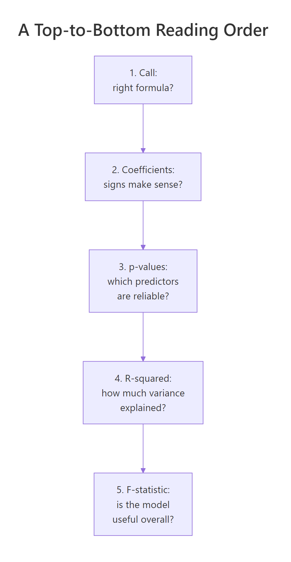
Figure 3: A quick top-to-bottom order for reading any lm() output.
The single most useful habit is to read every Estimate together with its Std. Error and p-value, never alone. That is the difference between a number you can act on and a number that is really just noise.
References
- R Core Team. summary.lm: Summarizing Linear Model Fits (R documentation). Link
- R Core Team. lm: Fitting Linear Models (R documentation). Link
- James, G., Witten, D., Hastie, T., Tibshirani, R. An Introduction to Statistical Learning, Chapter 3: Linear Regression. Link
- Wickham, H., Grolemund, G. R for Data Science, Model Basics. Link
- Faraway, J. Practical Regression and Anova using R. Link
- R Core Team. An Introduction to R, Chapter 11: Statistical models in R. Link
- Robinson, D. broom: Convert Statistical Objects into Tidy Tibbles. Link
Continue Learning
- Interpret lm() Output: Every Number Explained - a deeper companion that derives each statistic with the formulas behind it.
- Linear Regression in R - the full workflow from fitting a model to checking its assumptions.
- Logistic Regression in R - how to read model output when the outcome is yes or no instead of a number.