How to Read Logistic Regression Output in R
When you fit a logistic regression with glm(..., family = binomial) and call summary() on it, R prints a block of numbers that looks a lot like a linear-model summary but is not read the same way. This guide walks every line of that output, from the coefficient table down to the deviance and AIC, and shows how to turn each number into a plain statement about probability. Everything here uses base R, no extra packages.
Where should you look first in glm() output?
The hardest thing about a logistic summary is that its coefficients are not in the units you actually care about. Before we decode them, let's fit a real model and print the whole thing, so every later section has something concrete to point at. We will predict whether a car has a manual transmission (am, where 1 means manual and 0 means automatic) from its fuel economy (mpg), using the built-in mtcars data.
That is the whole printout. Press Run and it appears in a second. Now look at its shape rather than its numbers: it is a stack of labelled sections separated by blank lines, and each one answers a different question.
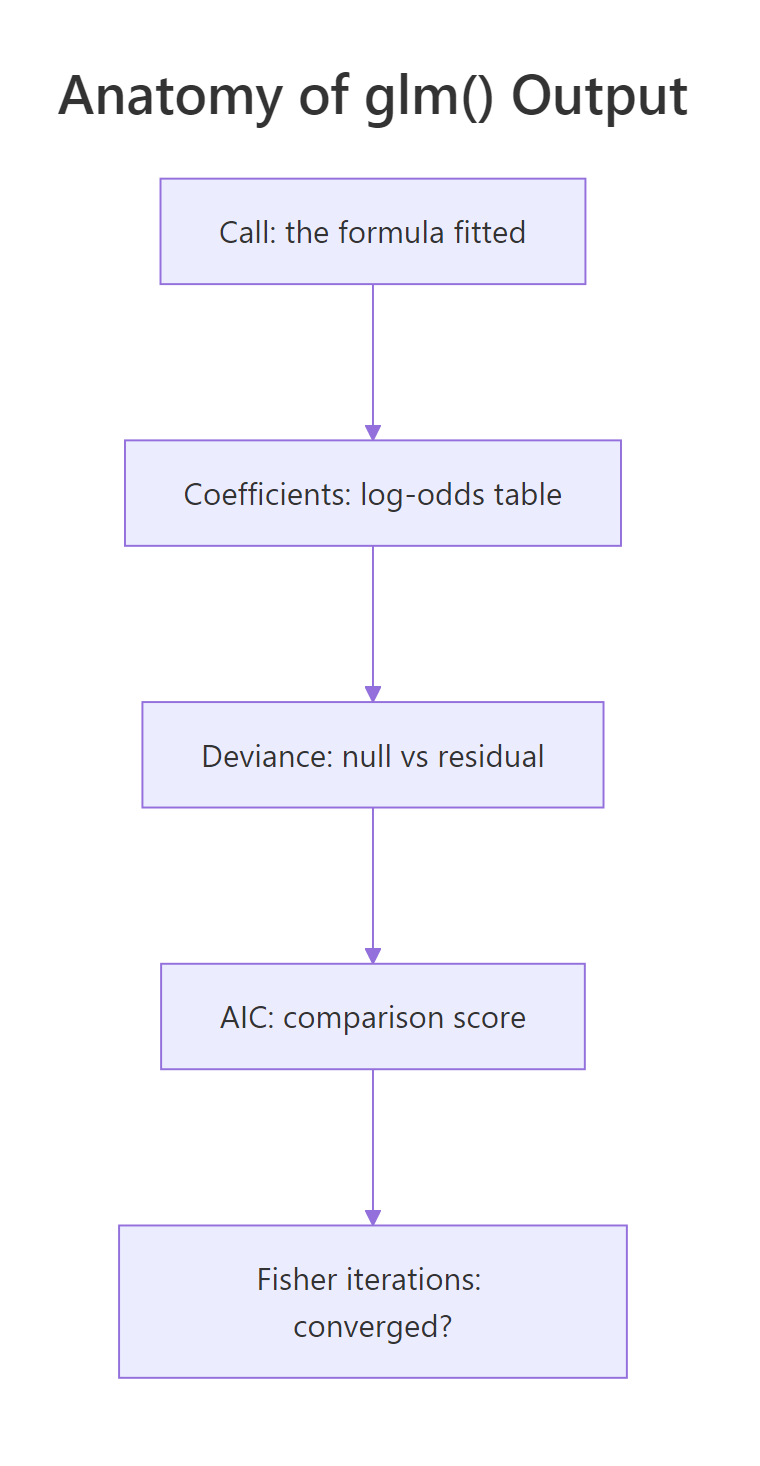
Figure 1: The stacked blocks of summary() output on a glm model.
Reading top to bottom, here is what each block is for:
- Call repeats the formula and family you fitted, so you can confirm R modelled what you meant.
- Coefficients is the heart of the output: the effect of each predictor, measured on a scale we will have to translate.
- Dispersion line is a one-line technical note that, for logistic regression, never changes.
- Null and Residual deviance compare your model against a do-nothing baseline.
- AIC is a single score for comparing whole models.
- Fisher Scoring iterations tells you the fitting routine finished cleanly.
We will walk through every block in that order. The rest of this guide is really just a magnified tour of this one printout.
Try it: Fit a model that predicts am from weight (wt) instead of fuel economy, then read its AIC.
Click to reveal solution
Explanation: AIC() pulls the single fit score straight out of the model. The weight model scores 23.18, lower than the fuel-economy model's 33.68, a first hint that weight predicts transmission type better. We will make that comparison properly later.
What is the Call line telling you?
The top block is the easiest to read and the easiest to skip, which is a mistake. The Call line simply echoes the formula, family, and data you handed to glm(). Its job is to let you confirm, at a glance, that R fitted the model you intended.
Let's pull the Call out on its own so you see it clearly.
This says the response is am, the single predictor is mpg, and the data came from mtcars. The tilde ~ reads as "is modelled by", so am ~ mpg means "am is modelled by mpg". The part that makes this logistic rather than linear is family = binomial. That one argument tells R the outcome is a yes-or-no event and switches it from fitting a straight line to fitting a probability curve.
Why does this matter? Because it is your receipt. If you meant to fit a logistic model but forgot the family argument, R would quietly fit an ordinary linear model instead, and the Call line is where you would catch it.
Try it: Fit a model of am on horsepower (hp) and read back its Call line to confirm both the formula and the family.
Click to reveal solution
Explanation: The Call confirms the predictor is hp and the family is binomial. Checking this one line prevents you from interpreting a model you did not mean to fit.
How do you read the coefficients table row by row?
This block holds the actual model estimates, so we will slow right down. The Coefficients table has one row per term (the intercept plus each predictor) and four columns. Let's print just the table, rounded, so nothing is hidden behind the stars.
Read it one column at a time.
The Estimate column is the number you came for, but here is the catch that trips up everyone new to logistic regression: this number is a change in log-odds, not a change in probability. The odds of an event are its chance of happening divided by its chance of not happening, and the log-odds are simply the natural logarithm of those odds. For the mpg row the estimate is 0.307, which means each extra mile per gallon adds 0.307 to the log-odds that a car is manual. The sign is the part you can read immediately: it is positive, so more fuel-efficient cars are more likely to be manual. The size, 0.307, only becomes meaningful after we translate it in the next section.
The (Intercept) row is the log-odds when every predictor is zero, so here it is the log-odds of a manual transmission for a car doing zero miles per gallon. A car cannot do zero mpg, so treat the intercept as the anchor point of the curve rather than a real forecast.
The Std. Error column measures how much the estimate would move if you collected the data again. A small standard error means the estimate is pinned down tightly. The mpg estimate of 0.307 has a standard error of 0.115, comfortably smaller than the estimate itself.
The z value column combines the two columns before it. It asks a simple question: how big is the estimate compared to its own uncertainty? You get it by dividing the Estimate by the Std. Error.
$$z = \frac{\hat{\beta}}{SE(\hat{\beta})}$$
Where:
- \\(\hat{\beta}\\) is the estimated coefficient (the Estimate column).
- \\(SE(\hat{\beta})\\) is its standard error (the Std. Error column).
Let's confirm the z value for mpg is really just that division.
That 2.67 matches the z value column exactly. This is the first place logistic output differs from a linear model: lm() reports a t value here, but glm() reports a z value, because the binomial model treats the spread as known rather than estimated. In practice you read them the same way, a value far from zero means a real effect.
The last column, Pr(>|z|), turns that z value into a probability, the p-value. It answers a cautious question: if this predictor truly had no effect, how often would random sampling alone hand us a z value this large? Let's read both p-values on their own.
The mpg p-value of 0.0075 means "this would almost never happen by luck", which is your evidence the effect is real. In the full printout R rounds these and adds a star key so you do not have to squint. Those are the significance codes:
***means the p-value is below 0.001 (strongest evidence).**means below 0.01.*means below 0.05, the usual cutoff for "statistically significant"..means below 0.10 (borderline).- a blank means above 0.10 (no real evidence).
Both rows earned **, so both are well supported by the data.
Try it: Rebuild the z value for the intercept the same way we did for mpg, straight from its Estimate and Std. Error.
Click to reveal solution
Explanation: The intercept's z value is -2.81, matching the printed table. unname() just drops the leftover label so you see a clean number. Every z value in the table is this same Estimate-over-Std.-Error division.
What do the coefficients mean as odds and probabilities?
We ended the last section with a coefficient nobody can act on: 0.307 log-odds per mpg. This section turns it into two things a human can actually say. A single coefficient lives on three connected scales, and moving between them is the core skill of reading logistic output.
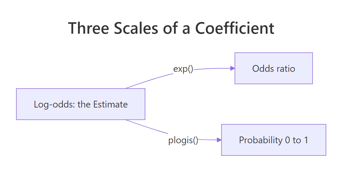
Figure 2: A logistic coefficient lives on three scales, running from log-odds to odds to probability.
The first jump is from log-odds to odds. Because the coefficient is a log-odds change, raising e to its power (the opposite of a logarithm) turns it into an odds ratio, the factor by which the odds multiply for a one-unit increase.
The mpg odds ratio is 1.36. Read it as: each extra mile per gallon multiplies the odds of a manual transmission by about 1.36, a 36 percent increase in the odds. An odds ratio above 1 means the predictor raises the odds and below 1 means it lowers them; a ratio of exactly 1 would mean no effect at all. The intercept's odds ratio (0.0014) is the baseline odds at zero mpg, which, like the intercept itself, is an anchor rather than a meaningful quantity.
exp(coef(model)) are what you actually say out loud to a colleague or a reader.Odds ratios are readable, but most people still think in probabilities. The link between them is the logistic equation, which says the log-odds are just a straight line built from the coefficients.
$$\log\left(\frac{p}{1-p}\right) = \beta_0 + \beta_1 x$$
Where:
- \\(p\\) is the probability the outcome is 1 (here, a manual car).
- \\(\frac{p}{1-p}\\) is the odds of that outcome.
- \\(\beta_0 + \beta_1 x\\) is the straight-line part, exactly like ordinary regression.
If you are not interested in the algebra, skip it. The practical point is that R will do the conversion for you. Asking predict() for the response gives you probabilities directly, one per car you describe.
A thirsty 15 mpg car has about a 12 percent chance of being manual; a frugal 25 mpg car has about a 75 percent chance. The type = "response" argument is what asks for probabilities; leave it out and R hands back raw log-odds instead. To prove the machinery, we can rebuild the 20 mpg probability by hand: plug the numbers into the straight line to get the log-odds, then run them through plogis(), which is R's name for the logistic curve that maps any log-odds back to a probability.
The 0.386 matches the middle prediction above exactly. That is the whole journey in one example: the coefficients give a log-odds, exp() turns a coefficient into an odds ratio, and plogis() turns a log-odds into a probability.
Finally, just as with a linear model, you can put a range around the odds ratios rather than trusting a single point. Exponentiating a confidence interval gives you the plausible range for each odds ratio.
The mpg odds ratio is most plausibly between 1.09 and 1.70. Because that whole range sits above 1, we are confident the effect is genuinely positive, which lines up with its small p-value. Whenever an odds ratio's interval straddles 1, that predictor is the shaky one.
Try it: Fuel economy usually changes by more than one mpg at a time. Work out the odds ratio for a 5 mpg increase.
Click to reveal solution
Explanation: Multiplying the coefficient by 5 before exponentiating gives the odds ratio for a 5 mpg jump: about 4.64. Five extra miles per gallon multiply the odds of a manual transmission more than fourfold, which is a far more tangible statement than the raw 0.307.
What do the deviance lines and AIC tell you about fit?
The bottom of the printout grades the model as a whole rather than one predictor at a time. There is no R-squared here, so these lines are how you judge overall fit. Let's start with the dispersion line, which reads (Dispersion parameter for binomial family taken to be 1). For logistic regression this is fixed and never changes, so you can read past it; it only becomes interesting for other model families.
The numbers that matter are the two deviances. Deviance measures how badly a model misses, so smaller is better. The Null deviance is the deviance of a model with no predictors at all, one that only knows the overall share of manual cars. The Residual deviance is what is left after your predictor does its work. The gap between them is the predictor's contribution. The "degrees of freedom" printed next to each deviance line is simply the number of cars minus the parameters the model fits: 31 for the null model (32 cars minus its single intercept) and 30 once mpg is added (minus the intercept and the mpg slope). Let's pull all three fit numbers out.
Adding mpg pulled the deviance down from 43.23 to 29.68, a drop of about 13.6. The natural next question is whether a drop that size is real or could have happened by chance. A drop-in-deviance test answers exactly that, comparing your model against the null.
The mpg row shows a deviance drop of 13.56 with a p-value of 0.00023, so fuel economy explains a genuinely useful chunk of the variation in transmission type. If you want a single number that feels like R-squared, McFadden's pseudo R-squared is the common choice: one minus the ratio of the two deviances.
This model gets about 0.31. Do not read pseudo R-squared like the real thing, though: McFadden values between 0.2 and 0.4 already indicate a good fit, so 0.31 is respectable. The last line of the printout, Number of Fisher Scoring iterations: 5, just reports that the fitting routine settled after five passes. Anything in the single digits is normal; a very large number, or a warning, is a sign the model struggled to converge.
Try it: You already fitted the weight model as ex_wt earlier, and it is still in memory. Compute its McFadden pseudo R-squared and compare it to the 0.31 above.
Click to reveal solution
Explanation: Weight scores 0.56, well above fuel economy's 0.31. Weight is the stronger single predictor of transmission type, which is the same story the lower AIC told us in the first section.
How does the output change with more than one predictor?
Real models almost always use several predictors. The good news is that the output keeps the same shape; the Coefficients table simply grows an extra row. Let's add horsepower to the fuel-economy model and read what changes.
There is now an hp row, and every coefficient's meaning shifts slightly: each one is now the effect of its predictor while holding the other predictor fixed. So the mpg coefficient is the log-odds change per mpg among cars of the same horsepower.
Notice the mpg coefficient jumped from 0.307 in the simple model to 1.260 here. That is not a bug. Fuel economy and horsepower are linked, powerful cars tend to burn more fuel, so in the one-predictor model the mpg coefficient absorbed part of horsepower's effect. Once horsepower is in the model and held fixed, fuel economy's own effect comes through more strongly. The odds ratios make the new scale concrete.
Holding horsepower fixed, each extra mpg now multiplies the odds of a manual transmission by 3.52, and each extra unit of horsepower multiplies them by 1.06. The model-fit lines improved too: residual deviance fell from 29.68 to 19.23, and AIC dropped from 33.68 to 25.23. Because AIC charges a penalty for each added predictor, a lower AIC after adding horsepower means the predictor genuinely earned its place.
anova(model1, model2, test = "Chisq") both weigh the improvement against the cost of the extra term.Try it: Add weight as a third predictor and see whether the AIC keeps dropping.
Click to reveal solution
Explanation: AIC fell again, from 25.23 to 16.77, so weight adds real predictive value on top of fuel economy and horsepower. Each drop in AIC is evidence the larger model is worth its extra complexity.
How do you go beyond summary(): predictions and accuracy?
The summary tells you about the coefficients, but the point of a classifier is usually to make calls on individual cases. predict() with type = "response" gives a probability for every car; turning those probabilities into yes-or-no predictions needs a cutoff, and 0.5 is the usual starting point. Comparing those predictions to the truth gives a confusion matrix.
Read the table by its diagonal. The model got 17 automatics and 7 manuals right, and missed 8 cars (2 automatics it called manual, 6 manuals it called automatic). Dividing the correct calls by the total gives overall accuracy.
The single-predictor model is right about 75 percent of the time. Before you trust any logistic model, run through this short red-flag checklist:
- A coefficient sign that makes no sense (fuel economy lowering the odds of a sporty manual) hints at a data or coding error.
- A standard error many times larger than its estimate is the classic sign of separation, where a predictor splits the outcome almost perfectly and the estimates blow up.
- A probability of exactly 0 or 1 for many cases, or coefficients in the tens or hundreds, is the same separation problem seen from a different angle.
- A large number of Fisher Scoring iterations, or a convergence warning, means the fitting routine struggled and the numbers may not be trustworthy.
Try it: Predict the probability of a manual transmission for a very frugal car doing 30 mpg.
Click to reveal solution
Explanation: The model puts a 30 mpg car's chance of being manual at about 93 percent. Note that 30 mpg sits near the top of the range in mtcars, so this is a reasonable extrapolation, but pushing much beyond the data would stop being trustworthy.
Practice Exercises
These pull together everything above. Each starter block runs as-is, so you can edit and rerun it until the output matches.
Exercise 1: Report an odds ratio with its interval
From a model of am on horsepower, report the odds ratio for hp together with its 95 percent confidence interval, then say whether horsepower is a reliable predictor on its own.
Click to reveal solution
Explanation: The hp odds ratio is 0.9919, and its interval (0.9802 to 1.0038) straddles 1. Because the interval crosses 1, horsepower alone is not a reliable predictor of transmission type, which is why you should always read an odds ratio next to its interval, never on its own.
Exercise 2: Choose between two models
Compare model A (am ~ mpg) with model B (am ~ mpg + hp) on both residual deviance and AIC, then say which model you would report.
Click to reveal solution
Explanation: Model B wins on both counts: lower residual deviance (19.23 versus 29.68) and lower AIC (25.23 versus 33.68). When a bigger model lowers the AIC, the drop in deviance is worth the extra predictor, so model B is the one to report.
Exercise 3: Rebuild a predicted probability by hand
For the two-predictor model am ~ mpg + hp, compute the predicted probability for a car with mpg = 25 and hp = 100 straight from the coefficients, then confirm it matches predict(). Use plogis() to turn the log-odds into a probability.
Click to reveal solution
Explanation: The by-hand probability and the predict() result agree to four decimals, both 0.9674. Building the log-odds from the coefficients and running them through plogis() is exactly what predict(type = "response") does internally, so reproducing it is the surest sign you understand the model.
Frequently Asked Questions
Why does my glm summary not show a Deviance Residuals block?
It was removed. R 4.1 stopped printing the five-number deviance-residual summary at the top of glm output, so on any modern R the printout jumps straight from the Call to the Coefficients. Older tutorials still show it, but you are not missing anything. If you want those residuals, residuals(model, type = "deviance") still returns them.
Are logistic regression coefficients the same as odds ratios?
No. The coefficients in the Estimate column are on the log-odds scale. You get the odds ratio by exponentiating them with exp(coef(model)). This is the most common source of misreadings, so always check which scale a number is on before you interpret it.
Why does glm report a z value when lm reports a t value?
Because the binomial model treats the outcome's variability as known rather than estimated from the data. That changes the reference distribution for each coefficient's test from a t distribution to a standard normal one, which is why the column is labelled z value and the p-value column is Pr(>|z|). You read them the same way you read t values.
What counts as a good AIC or deviance value?
There is no absolute target. AIC and deviance are only meaningful when you compare models fitted to the same data, where lower is better. A single AIC of 25 is neither good nor bad on its own; it only matters that another model scores higher or lower.
Why is one of my coefficients huge with an enormous standard error?
That is the classic signature of separation, where a predictor splits the two outcomes almost perfectly. The model tries to push that coefficient toward infinity, and both the estimate and its standard error balloon. When you see it, the fix is usually to drop or combine the offending predictor, or to use a penalized method built for separation.
Summary
Reading glm() output is a matter of taking it block by block and knowing what question each line answers, plus one extra skill the linear model never needed: translating coefficients off the log-odds scale. Here is the whole tour on one card.
| Line in the output | What it answers | ||
|---|---|---|---|
| Call | Did R fit the formula, data, and family I intended? | ||
| Estimate | How much does each predictor move the log-odds, and in which direction? | ||
| Std. Error | How precise is that estimate? | ||
| z value | How many standard errors is the estimate from zero? | ||
| Pr(> | z | ) and stars | Could this effect be luck, or is it well supported? |
| exp(coef) | The odds ratio: the readable version of the coefficient. | ||
| Null deviance | How badly does a no-predictor baseline miss? | ||
| Residual deviance | How badly does my model miss after the predictors? | ||
| AIC | Which of two models fits better, penalizing extra terms? | ||
| Fisher Scoring iterations | Did the fitting routine converge cleanly? |
When you open a new logistic summary, this order works well.

Figure 3: A quick top-to-bottom order for reading any glm() output.
Confirm the Call, check each coefficient's sign against common sense, scan the p-values for which predictors are reliable, exponentiate to talk in odds ratios, and read the deviance and AIC to judge the model overall. The single most useful habit is to translate before you interpret: a raw log-odds coefficient is for the math, but an odds ratio or a predicted probability is what you actually report.
References
- R Core Team. glm: Fitting Generalized Linear Models (R documentation). Link - the reference for every argument in the
glm()call, including the family options. - R Core Team. summary.glm: Summarizing Generalized Linear Model Fits (R documentation). Link - documents exactly what each column and line of the summary you are reading contains.
- R Core Team. predict.glm: Predict Method for GLM Fits (R documentation). Link - explains the
type = "response"argument that turns log-odds into probabilities. - James, G., Witten, D., Hastie, T., Tibshirani, R. An Introduction to Statistical Learning, Chapter 4: Classification. Link - a free, readable textbook treatment of logistic regression and how to interpret it.
- UCLA OARC Statistics. Logit Regression: R Data Analysis Examples. Link - a worked logistic example with odds ratios, confidence intervals, and predicted probabilities.
- Faraway, J. Extending the Linear Model with R: Generalized Linear, Mixed Effects and Nonparametric Regression Models. Link - a deeper reference on generalized linear models and their diagnostics.
- R Core Team. An Introduction to R, Chapter 11: Statistical models in R. Link - the official R introduction to fitting models with formulas, including
glm().
Continue Learning
- How to Read lm() Output in R Line by Line - the same block-by-block treatment for ordinary linear regression, a useful companion to this guide.
- Logistic Regression in R - the full workflow from fitting a logistic model to evaluating and using it.
- Linear Regression in R - where regression starts, with a numeric outcome instead of a yes-or-no one.