Power Analysis by Simulation in R
Power analysis by simulation estimates your study's chance of detecting a real effect: you generate many fake datasets under an assumed effect, run your test on each one, and count how often it comes out significant. That share is your power. The huge advantage is that it works for any design, even ones no formula covers. Everything below is plain base R.
What does statistical power actually mean?
Imagine there really is a difference between two groups, and you run a study to catch it. Sometimes your data will show a clear, significant result. Other times, by bad luck, the same true difference will slip through and your test will come up empty. Statistical power is simply how often you would catch that real effect if you could repeat the study over and over.
Put formally, power is the probability that your test returns a significant result when the effect is genuinely there. It is the flip side of a miss. When a real effect exists but your test fails to flag it, that is a false negative, also called a Type II error. Power and the miss rate always add up to one.
$$\text{Power} = 1 - \beta$$
Where $\beta$ (beta) is the Type II error rate, the chance of missing a real effect. A study with 80% power misses a true effect 20% of the time.
There is a second way a test can go wrong, and it helps to name both together. A false alarm, where you declare a significant result even though nothing is really going on, is a Type I error. You control its rate directly with your significance threshold, usually $\alpha = 0.05$. The diagram below lays out all four things that can happen.
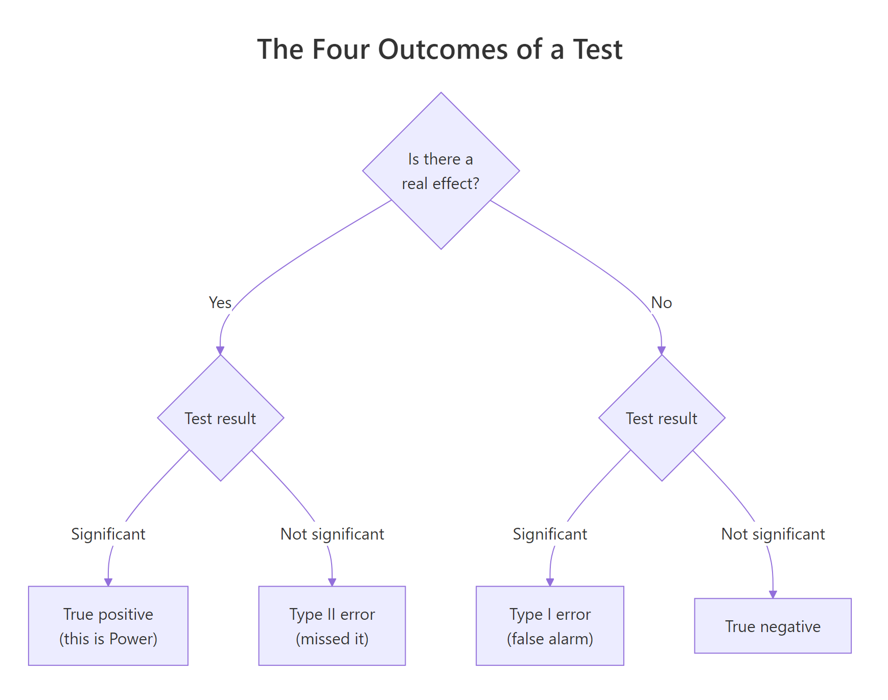
Figure 1: The four outcomes of a test. Power is the top-left cell, a real effect correctly detected.
Power is driven by four levers, and every power analysis is really a conversation about them:
- Sample size. More data means more power. This is usually the lever you control.
- Effect size. Bigger true differences are easier to detect.
- Significance level (alpha). A stricter threshold makes significance harder to reach, lowering power.
- Variability. Noisier data makes a real difference harder to detect, which lowers power.
Let us make this concrete. Suppose a control group has a true average of 100 and a treatment truly lifts it to 105, a real 5-point effect, with a standard deviation of 15 in both groups. We will draw 30 people per group and run a two-sample t-test. Before reading the result, ask yourself: with a real effect present, will the test catch it?
Here is what happened. The rnorm(30, mean = 100, sd = 15) call drew 30 random values from a normal distribution centred at 100, our stand-in for a control group. The second call did the same but centred at 105, the treatment group that truly is 5 points higher. The t.test() then compared the two groups and returned a p-value of 0.09.
That p-value is above 0.05, so this particular experiment failed to reach significance. Read that again: the effect is real, we built it into the data ourselves, yet this one study missed it. A single experiment is a coin flip with weighted odds. It cannot tell you your power, because it is just one draw from a noisy process.
Try it: A bigger true effect should be easier to detect. Change the treatment mean from 105 to 115 (a 15-point lift) and rerun the same test. Does the p-value now drop below 0.05?
Click to reveal solution
Explanation: A 15-point lift is three times the earlier effect, so the two groups separate cleanly and the p-value falls to 0.014, comfortably below 0.05. Larger effects are easier to catch, which is lever number two in action.
How do you estimate power by simulating many experiments?
If one experiment is a coin flip, the fix is obvious: flip the coin many times and count. That is the entire idea behind power analysis by simulation. You assume an effect, simulate a full dataset, run your test, note whether it reached significance, and then repeat that hundreds or thousands of times. The share of runs that came out significant is your estimated power.
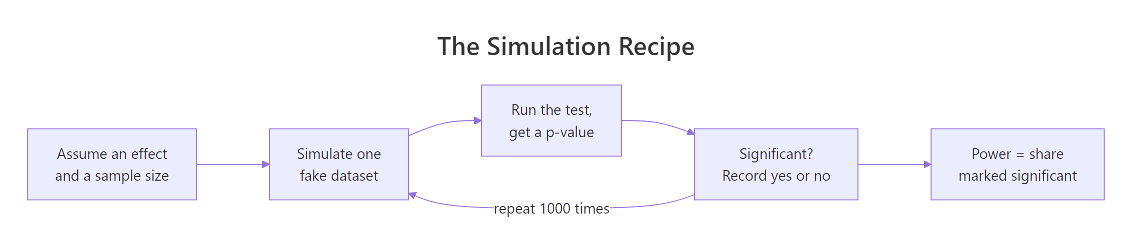
Figure 2: The simulation recipe. Assume an effect and a sample size, simulate a dataset, run the test, record whether it was significant, and repeat before averaging.
R gives us a clean tool for "do this many times and collect the answers": replicate(). You hand it a number of repetitions and a block of code, and it runs that block that many times, gathering each result into a vector. We will run our 5-point experiment 1000 times and, on each run, record TRUE when the p-value beats 0.05 and FALSE when it does not.
Walk through what this did. Inside the curly braces we rebuilt the same two groups from before, then asked one yes-or-no question: is the p-value below 0.05? That comparison returns TRUE or FALSE. replicate() ran the block 1000 times and stacked those 1000 answers into reject. Taking mean() of a TRUE/FALSE vector gives the proportion of TRUE values, because R treats TRUE as 1 and FALSE as 0.
The number is low. With a real 5-point effect, 30 people per group, and this much noise, the test only catches the effect about 23% of the time. More than three studies out of four would come back non-significant despite the effect being real. That is a badly underpowered design, and simulation told us so before we spent a cent collecting data.
Now, how do we know 0.234 is trustworthy and not a bug in our loop? For this simple two-sample t-test, a classical formula exists, and R ships it as power.t.test(). We can compute the exact analytic power for the same setup and compare.
The formula says 0.245; our simulation said 0.234. They agree to within the noise of 1000 runs. That agreement is the whole reason simulation is safe to trust.
Try it: Doubling the sample size should raise power. Re-estimate power with 60 people per group instead of 30, keeping the same 5-point effect. Fill in the significance check inside the loop.
Click to reveal solution
Explanation: Doubling the group size lifts power from about 0.23 to about 0.43. More data sharpens the estimate of each group's mean, so a real gap is easier to distinguish from noise. Still short of the usual 0.80 target, which is exactly the question we tackle next.
How many participants do you need for 80% power?
Most of the time you already know the effect you care about and the noise you expect. The real question is planning: how large does the study need to be to hit a power you would be comfortable with, usually 0.80? To answer that, we turn the simulation into a reusable function of sample size, then try a range of sizes and see where power crosses the line.
First, the function. It takes a per-group sample size n and returns the estimated power. The effect (delta), noise (sd), and number of simulations (n_sim) get sensible defaults so we can call it with just a sample size.
The body is the same loop as before, just wrapped so we can vary n. Calling power_for_n(30) reproduces our earlier answer of about 0.25, which confirms the function works. Now the payoff: feed it a whole range of sample sizes at once. The sapply() function applies power_for_n to each value in a vector and collects the results, so we get one power estimate per candidate sample size.
Reading down the table, power climbs steadily with sample size, as expected. It crosses 0.80 somewhere between 140 and 160 per group. Rather than eyeball it, let us ask R for the first sample size that reaches our target.
The which(power_curve >= 0.80) part finds the positions where power meets or beats 0.80, and [1] grabs the first of them. Indexing sample_sizes at that position returns 160. So on this grid, 160 people per group is the smallest size that clears 80% power. The true crossing sits near 142, but our grid steps by 20, so 160 is the first candidate that qualifies.
A picture makes the trade-off obvious. Plotting the curve with a reference line at 0.80 shows exactly where the design becomes adequately powered.
The rising curve flattens as it climbs, which is why chasing very high power gets expensive: each extra bit of power near the top costs more and more participants.
Try it: Aiming higher costs more. Reuse power_for_n() to find the smallest sample size that reaches 90% power for the same 5-point effect.
Click to reveal solution
Explanation: Reaching 90% power needs about 200 per group, up from 160 for 80%. That extra 10 percentage points of power costs roughly 40 more people in each group, a clear picture of how steep the top of the curve is.
Why simulate instead of using a power formula?
If power.t.test() already exists, why bother simulating? Because that formula, and the tidy ones in packages, quietly assume a perfect world: two groups of equal size, equal variances, and neatly normal data. Real studies rarely oblige. The moment your design steps outside those assumptions, the formula either does not exist or silently answers a slightly different question than the one you are asking.
Simulation has no such limits. You simulate data the way you actually believe it behaves, and you run the exact test you plan to run. Consider a common wrinkle: the two groups have different amounts of spread. Say the control group has a standard deviation of 10 but the treatment response is much more variable, with a standard deviation of 25. The everyday two-sample t-test in R (the Welch version) already handles unequal variances, so we simulate that scenario and run it directly.
With 40 per group and a 6-point effect, but one very noisy group, power is only about 0.26. A naive equal-variance formula fed the average spread would report a higher power, because it ignores that the treatment group is so much more variable. The simulation used the true, unequal noise levels and the actual Welch test you would run, so its answer reflects your real study.
Try it: Outcomes like income or reaction time are often skewed, not normal, and are frequently analysed with a rank-based test. Simulate a skewed outcome using rlnorm() (which draws from a right-skewed lognormal distribution) and test it with wilcox.test() instead of a t-test.
Click to reveal solution
Explanation: Swapping in a skewed outcome and a different test changed exactly one line inside the loop, and the recipe carried on unchanged. Power came out around 0.48. No standard formula covers "lognormal outcome tested with a Wilcoxon test", yet simulation handles it directly.
How do you simulate power for a regression slope?
Notice a pattern in every example so far: only the middle of the loop ever changed. We always simulate data, run a test, and extract a p-value; the surrounding "repeat and average" scaffolding stays put. That is why the same recipe scales to designs far beyond two-group comparisons. To prove it, let us leave t-tests entirely and estimate power to detect a slope in a regression.
Here the effect is a slope. We will simulate a predictor x, build an outcome y that truly depends on it through the line y = 2 + 0.3 * x plus random noise, fit a linear model with lm(), and check whether the slope on x is significant. The only new trick is pulling the p-value out of the model summary.
The line coef(summary(model))["x", "Pr(>|t|)"] reaches into the model's coefficient table and grabs the p-value for the x row, the column labelled Pr(>|t|). Everything else is the familiar loop. With 80 observations and a true slope of 0.3 against noise of 1, we would detect the slope about 75% of the time. If that is not enough, you already know the fix: raise the sample size and rerun.
coef(summary(model)). For a fitted model, coef(summary(model)) returns the coefficient table with estimates, standard errors, and p-values. Index the row by predictor name and the column by "Pr(>|t|)" to pull out exactly the p-value your power loop needs.Try it: Weaker effects are harder to detect. Lower the true slope from 0.3 to 0.15, keep everything else the same, and re-estimate power.
Click to reveal solution
Explanation: Halving the slope more than halves the power, from about 0.75 down to 0.28. Small effects demand much larger samples, and simulation quantifies exactly how much larger before you commit to the study.
What mistakes make a power simulation wrong?
Simulation is powerful, but a few traps can hand you a confident wrong answer. The first is running too few repetitions. A power estimate is itself a statistic, computed from a finite number of runs, so it carries its own uncertainty. That wobble, the Monte Carlo error, shrinks as you add simulations, following the same square-root rule as any proportion.
$$\text{SE} \approx \sqrt{\frac{\hat{p}\,(1-\hat{p})}{n_{\text{sim}}}}$$
Where $\hat{p}$ is your estimated power and $n_{\text{sim}}$ is the number of simulations. The table below shows how the standard error of a power estimate near 0.80 tightens as you crank up the repetitions.
At 100 runs the estimate can drift by 4 percentage points, enough to flip a "0.80" into a "0.76" or "0.84" purely by chance. At 1000 runs the wobble drops to about 1.3 points, and at 10000 runs to well under half a point. Use at least 1000 simulations for a working estimate, and 10000 for a final number you will report.
The second trap is more subtle and more dangerous: guessing the effect size wrong. Simulation cannot invent the truth, it can only propagate the effect you assume. Feed it an optimistic guess and it hands back an optimistic power. The honest habit is to plug in the smallest effect that would still matter to you, not the largest you hope for, so your study is powered for the outcome you actually care about.
Finally, always call set.seed() before a power simulation. It makes your result reproducible, so a colleague running your script gets the same number and can check your reasoning rather than a different random draw.
Try it: Quantify the wobble directly. A simulation of 1000 runs returns an estimated power of 0.62. Build an approximate 95% Monte Carlo interval for it using the formula above (estimate plus or minus 1.96 standard errors).
Click to reveal solution
Explanation: The true power plausibly sits between 0.59 and 0.65 given only 1000 runs. If you need to pin it down more tightly, the only lever is more simulations, which narrows the interval by the square-root rule.
Complete example: planning a two-group study end to end
Let us put every piece together on a realistic decision. You are testing two versions of a web page and the outcome is time on page, measured in seconds. Past data suggests a control average near 100 seconds with a standard deviation of about 20. You would only care about a lift of 6 seconds or more, so that is the smallest effect worth powering for. The question your manager asks: how many visitors per version do we need for 80% power?
We already have the tool. power_for_n() accepts delta and sd, so we just point it at this scenario, delta = 6 and sd = 20, and sweep a grid of sample sizes.
Power passes 0.80 at 175 visitors per version. Let us read that off directly rather than trusting a glance at the table.
So the plan is 175 visitors per version, 350 in total. Because this is a plain two-group comparison with equal variances, a formula also exists here, which gives us one last chance to sanity-check the whole workflow.
The formula agrees almost exactly: 0.799 against our simulated 0.801. You now have a defensible, reproducible sample size, and the same script would have worked even if the design had unequal groups or a skewed outcome where no formula applies.
Practice Exercises
These combine several ideas from the tutorial. Each uses distinct variable names so your code will not clobber the tutorial's variables. Try each before opening the solution.
Exercise 1: Power with unequal group sizes
Recruitment is uneven: you can enroll 40 people in the control group but 80 in the treatment group. The true effect is a 5-point lift and the standard deviation is 15 in both groups. Estimate the power of a two-sample t-test for this unbalanced design using 2000 simulations.
Click to reveal solution
Explanation: The unbalanced design reaches about 0.39 power. Extra treatment-group participants help, but a study is limited by its smaller group, so 40 control participants cap the gains. Simulation handles the imbalance with no special formula.
Exercise 2: Power for a one-way ANOVA
You have three groups with true means of 100, 103, and 107, a shared standard deviation of 12, and 30 people in each group. Estimate the power of a one-way ANOVA to detect that the groups differ at all, using its overall F-test. Use 2000 simulations. Hint: build the outcome with c(), label the groups with factor(rep(...)), and pull the p-value from summary(aov(y ~ g))[[1]][["Pr(>F)"]][1].
Click to reveal solution
Explanation: The design has about 0.50 power, only a coin flip's chance of detecting the group differences. The same recipe extends past two groups: only the data-building and test lines changed, while the repeat-and-average scaffolding stayed identical.
Exercise 3: Power for a two-proportion test
A conversion rate is 30% on the current page and you hope a redesign lifts it to 45%. With 100 visitors per version, estimate the power of a two-proportion test using 3000 simulations, then compare your answer to power.prop.test(). Hint: draw counts with rbinom(1, 100, p) and test them with prop.test(c(x1, x2), c(100, 100), correct = FALSE).
Click to reveal solution
Explanation: The simulation returns about 0.585 and the formula about 0.592, a close match that validates the approach on yet another design. At 100 per version this test has only around 59% power, so you would want more visitors before trusting a non-significant result.
Frequently asked questions
How many simulations do I need?
Use at least 1000 runs for a working estimate and 10000 for a number you will report or defend. The reason is Monte Carlo error: a power estimate is itself computed from a finite number of runs, so it varies. As the Monte Carlo error table showed, 1000 runs pin the estimate to about one percentage point and 10000 runs to under half a point.
Is simulated power as trustworthy as a formula?
Yes, when the formula's assumptions actually hold. Every time we could check, the simulation matched power.t.test() and power.prop.test() to within the noise of a few thousand runs. The advantage of simulation is that it keeps working for designs no formula covers, like unequal variances or a skewed outcome analysed with a rank-based test.
What effect size should I plug in?
Use the smallest effect that would still matter to you, not the largest you are hoping for. Simulation only propagates the effect you assume, so an optimistic guess yields an optimistically high power and an underpowered study. Never run the study first and feed the observed effect back in; that "post-hoc power" is just your p-value restated.
Why do I get a slightly different power each time I run it?
Because each run draws fresh random data, so the estimate moves from one execution to the next. Call set.seed() before the simulation to make the result reproducible, and raise the number of simulations to shrink the run-to-run variation.
Can I use this for tests other than the t-test?
Yes. Only the middle of the loop changes: simulate your data, run whatever test you plan to use, then record whether its p-value beat your threshold. The same scaffolding handled a regression slope, a one-way ANOVA and a two-proportion test earlier in this post.
Summary
Power analysis by simulation replaces hard-to-remember formulas with one repeatable recipe: assume an effect, simulate data, run your test, and count how often the test reaches significance. Because you simulate the data and run the test you actually plan to use, the method stretches to any design, including the messy ones no formula covers.
| Idea | What to remember |
|---|---|
| Power | The long-run chance of detecting a real effect, equal to 1 minus the Type II error rate |
| The recipe | Simulate a dataset, run the test, record significance, repeat, then average |
replicate() |
Runs the simulation block many times and collects the significance flags |
| Sample size | Sweep a grid of sizes to find the smallest one that hits your target power |
| Any design | Only the simulate-and-test core changes; t-test, regression, ANOVA all reuse the loop |
| Monte Carlo error | Power estimates wobble; use 1000+ runs, and 10000 for a reported number |
| Effect size | Power for the smallest effect that matters, and never compute post-hoc power |
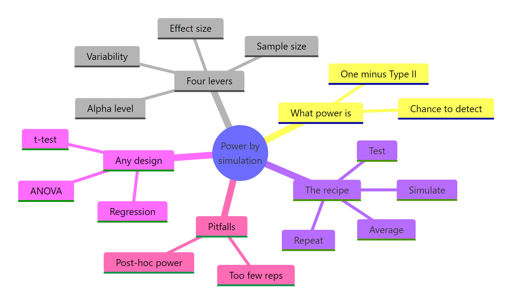
Figure 3: Power by simulation at a glance: what power means, the simulation recipe, the designs it handles and the pitfalls to avoid.
References
- R Core Team. power.t.test: Power Calculations for Two-Sample t Tests (stats package documentation). Link
- Cohen, J. Statistical Power Analysis for the Behavioral Sciences, 2nd Edition. Routledge (1988). The foundational text on effect sizes and power.
- Green, P. & MacLeod, C. J. SIMR: an R package for power analysis of generalized linear mixed models by simulation. Methods in Ecology and Evolution, 7(4), 493-498 (2016). Link
- Ford, C. Power and Sample Size Analysis using Simulation. University of Virginia Library, StatLab. Link
- Gelman, A. & Hill, J. Data Analysis Using Regression and Multilevel/Hierarchical Models. Cambridge University Press (2007). Chapter on fake-data simulation for design and power.
- R Core Team. An Introduction to R (probability distributions and
replicate). Link - Champely, S. pwr: Basic Functions for Power Analysis (vignette). Link
Continue Learning
- Statistical Power Analysis in R: the formula-based companion to this post, using closed-form power functions for standard designs.
- Sample Size Planning in R: a broader look at deciding how many observations your study needs before you collect data.
- Type I and Type II Errors in R: a closer look at false alarms and misses, the two error types that power is built from.