Z-Scores and Percentiles in R
A z-score tells you how many standard deviations a value sits above or below the mean. A percentile tells you what fraction of the data falls below that value. This tutorial builds both from scratch in base R, then shows you how to convert between them and where each one can quietly mislead you.
Why do raw numbers lie, and what fixes them?
Imagine a student who scored 80 in a math test and 65 in a reading test. The 80 looks better. But suppose the math class averaged 70 and the reading class averaged 55, and reading scores were far more tightly packed. Once you know how each class performed, the ranking can flip. Raw numbers measured on different scales are not directly comparable, and a z-score is the tool that fixes that.
A z-score rescales any value onto one common ruler: its distance from the mean, measured in standard deviations. Let's compute both scores the same way and see which result is actually more impressive.
Here is what the code did. For each subject we subtracted the class mean from the student's score, then divided by that class's standard deviation. Math gives 1.25 and reading gives 2.50.
Now the interpretation. The 80 in math is 1.25 standard deviations above its class average, but the 65 in reading is a full 2.50 standard deviations above its class average. Relative to their peers, the reading result is the standout, even though its raw number is lower. That reversal is the whole point of standardizing.
The formula behind the two lines above is short. When you know the true population mean and standard deviation, the z-score of a value $x$ is:
$$z = \frac{x - \mu}{\sigma}$$
Where:
- $x$ = the value you are scoring
- $\mu$ = the mean of the group (the Greek letter mu)
- $\sigma$ = the standard deviation of the group (the Greek letter sigma)
In practice you almost never know the true population values, so you estimate them from a sample. The sample version swaps in the sample mean $\bar{x}$ and the sample standard deviation $s$:
$$z = \frac{x - \bar{x}}{s}$$
The sign and size of a z-score are easy to read once you know the pattern.
| Z-score | What it means |
|---|---|
| 0 | exactly at the mean |
| +1 | one standard deviation above the mean |
| -2 | two standard deviations below the mean |
| 3 or more (either sign) | unusually far out, a possible outlier |
Try it: A student scored 66 in a science test where the class mean was 60 and the standard deviation was 4. Work out the z-score by hand in R.
Click to reveal solution
Explanation: The score is 6 points above the mean, and each standard deviation is worth 4 points, so 6 divided by 4 gives a z-score of 1.5.
How do you compute z-scores in R with scale()?
Doing the arithmetic by hand is fine for one number, but real data comes in whole columns, and you rarely know the mean and standard deviation in advance. You compute them from the data itself. R has a built-in function, scale(), that centers and standardizes a vector in one step.
Let's set up a small class of twelve students with math and reading scores. We will standardize these columns and keep using this data frame for the rest of the tutorial.
Now hand the math column to scale(). Watch the output carefully, because it is not a plain vector.
Two things happened. First, scale() returned a single-column matrix, not a vector, which is why every row is printed with a [1,] style index. Second, it attached two useful numbers at the bottom: scaled:center is the mean it subtracted (74.83) and scaled:scale is the standard deviation it divided by (11.84). So scale() computed the mean and standard deviation from your data automatically.
as.numeric() to get a clean numeric vector.Let's do exactly that and round the result so it is easy to read.
Ana's 82 becomes a z-score of 0.61 here. Notice that back in the opening section a score of 80 gave a z-score of 1.25, because that was a different class with a lower average. Same idea, different reference group, different z-score.
A standardized column always has the same two properties: its mean is 0 and its standard deviation is 1. That is what "standard" refers to. Let's confirm it.
The mean comes back as 0 and the standard deviation as 1, exactly as promised. You can also standardize several columns in one call by passing a data frame of numeric columns.
Each column is standardized on its own terms, using its own mean and standard deviation. Ana (row 1) is 0.61 standard deviations above average in math and 0.66 above in reading, so she is slightly stronger in reading relative to her class.
sd() uses, which is the right choice when your data is a sample rather than the entire population. If you ever need the population version, divide by your own hand-computed population standard deviation instead.Try it: Standardize the reading column into a clean numeric vector and round it to two decimals.
Click to reveal solution
Explanation: scale() centers and standardizes the reading column, and as.numeric() strips the matrix wrapper so you get a plain vector.
What is a percentile, and how do you read it off your data?
A percentile answers a ranking question: what fraction of the data falls at or below a given value? If a score is at the 90th percentile, 90 percent of the values are at or below it. Percentiles are intuitive because they need no assumptions, they just count positions in your actual data.
There are two directions you might want to go, and R has a function for each. Use quantile() when you have a percentile and want the value at it. Let's find the values at the 25th, 50th, 75th, and 90th percentiles of the math scores.
The output reads directly: a quarter of the class scored 67.25 or below, half scored 73 or below (that is the median), and the top ten percent starts around 89.8. Each label on top is the percentile, and each number beneath is the score at that cut point.
The other direction is more common in practice: you have a value and want its percentile. Use ecdf(), which stands for empirical cumulative distribution function. It builds a function that, given a value, returns the proportion of the data at or below it.
The line ecdf(students$math) builds the ranking function, and calling it on 82 returns 0.75. That means 75 percent of the class scored 82 or below, so a score of 82 sits at the 75th percentile of this group.
You can hand the whole column back to the same function to get everyone's percentile at once. Multiplying by 100 turns the proportions into familiar percentile numbers.
Every student now has a percentile rank. Lena, with the top score of 95, lands at the 100th percentile, while Eli's 58 sits at the 8th. These ranks come purely from counting positions in this class, with no formula about shapes or curves involved.
type argument.Try it: Find the reading score that marks the 80th percentile of the class.
Click to reveal solution
Explanation: Passing a single probability of 0.80 asks quantile() for the value below which 80 percent of the reading scores fall.
How do you convert a z-score to a percentile (and back)?
So far z-scores and percentiles have felt like separate tools. They are actually two views of the same idea, and R lets you move between them with a pair of functions built around the standard normal distribution, the familiar bell curve with mean 0 and standard deviation 1.

Figure 1: The path from a raw value to a percentile, and back with qnorm().
To go from a z-score to a percentile, use pnorm(). It returns the proportion of a normal distribution that lies below a given z-score. Let's convert a z-score of 1.5.
A z-score of 1.5 corresponds to 0.9332, so it sits at roughly the 93rd percentile of a normal distribution. About 93 percent of a bell-shaped population would fall below a value that is 1.5 standard deviations above the mean.
To go the other way, from a percentile to the z-score that marks it, use qnorm(). It is the exact inverse of pnorm(). Let's find the z-score at the 90th percentile.
The 90th percentile of a normal distribution sits at a z-score of about 1.28. Feed that 1.28 back into pnorm() and you would land on 0.90 again, which is what "inverse functions" means.
Now let's run the full pipeline on real data: take Ana's math score of 82, standardize it against her class, and read off its theoretical percentile.
The score of 82 is 0.61 standard deviations above the class mean, and pnorm() places that at the 72.8th percentile. Earlier, counting positions directly with ecdf() put the same 82 at the 75th percentile. The two answers are close here because this small class is fairly symmetric, but they are computed in completely different ways, and later you will see them disagree.
The normal distribution also explains the famous 68-95-99.7 rule. Let's derive it with pnorm() by measuring how much of the curve lies within one, two, and three standard deviations of the mean.
Subtracting the percentile at the lower bound from the percentile at the upper bound gives the share of values in between. About 68 percent of a normal distribution falls within one standard deviation of the mean, 95 percent within two, and 99.7 percent within three. That is why a z-score beyond 3 is treated as rare.
Try it: Find the z-score at the 95th percentile with qnorm(), and the percentile of a z-score of -1 with pnorm().
Click to reveal solution
Explanation: The 95th percentile sits at a z-score of about 1.64, and a z-score of -1 (one standard deviation below the mean) sits at about the 16th percentile.
Empirical vs theoretical percentiles: which should you trust?
The two paths to a percentile in the last section were not interchangeable, and the difference matters enormously the moment your data stops being bell-shaped. This is the point most tutorials skip, and it is the one that will save you from wrong conclusions.
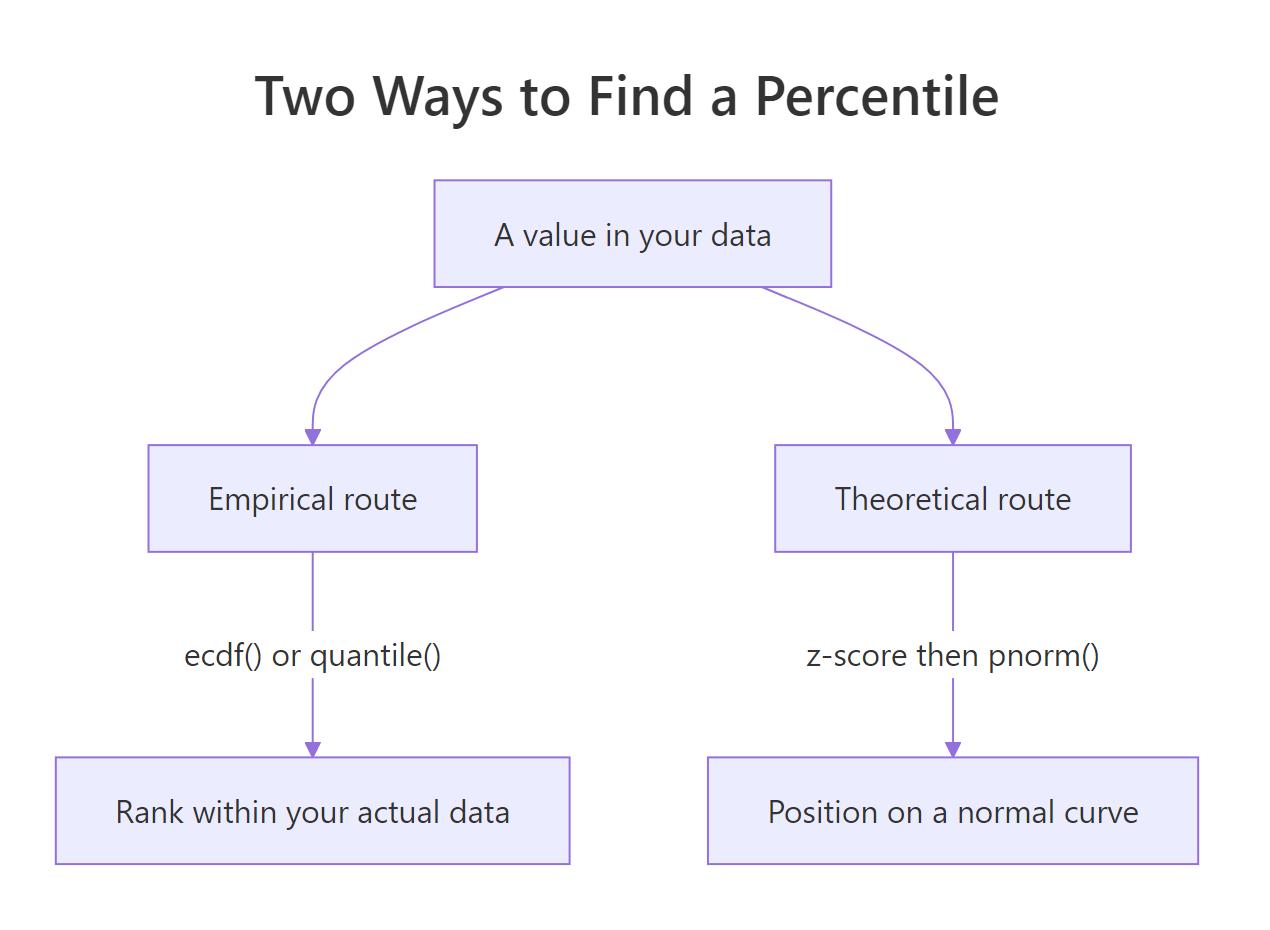
Figure 2: Two routes to a percentile: from your actual data, or from a normal model.
There are two kinds of percentile. An empirical percentile comes from ecdf() or quantile(), which count positions in your real data and assume nothing about its shape. A theoretical percentile comes from converting a z-score with pnorm(), which assumes your data follows a normal curve. When the data really is bell-shaped, the two agree. When it is skewed, they can be far apart.
Let's build a clearly skewed sample: household incomes, which have a long right tail because a few people earn a lot. We simulate 1000 incomes and look at the center. The set.seed() call fixes the random draw so you get the same numbers shown here.
The mean income (48,308) is far above the median (33,718). That gap is the signature of right skew: a handful of very high earners pull the average up, while most people sit below it. Now watch what happens when we ask where the average earner ranks.
Here is where the two methods disagree. Because the mean always has a z-score of 0, pnorm() insists the mean sits at the 50th percentile, as it would for any normal distribution. But counting the actual data, the mean income sits at the 64th percentile: 64 percent of households earn at or below the average. The theoretical answer is simply wrong for this data, because incomes are not normal.
pnorm() only gives a correct percentile when your data is roughly bell-shaped. For skewed data, trust ecdf() and quantile(), which read percentiles straight from the values you actually have.Try it: For an income of 90,000, compute both the empirical percentile (with ecdf()) and the theoretical percentile (standardize, then pnorm()), and see how far apart they land.
Click to reveal solution
Explanation: The empirical percentile counts that 85.7 percent of incomes are at or below 90,000, while the normal-based estimate says only 80.3 percent. The gap is the skew showing through, and the empirical number is the honest one for this data.
How do you use z-scores to spot outliers?
A popular rule of thumb flags any value with a z-score beyond 3 as an outlier, since the 68-95-99.7 rule showed that only 0.3 percent of a normal distribution lies out there. It is a handy first pass, but it has a trap you should see before you rely on it.
Consider ten temperature readings where one sensor glitched and reported 95 instead of a normal room temperature. Let's compute standard z-scores and check the largest.
The glitch value of 95 gets a z-score of only 2.84, which is below the threshold of 3. The rule misses it. This happens because the outlier is so extreme that it inflates the very mean and standard deviation used to score it, which lowers its own z-score back below the threshold. Statisticians call this masking.
The fix is a robust z-score that uses measures the outlier cannot distort. Swap the mean for the median and the standard deviation for the median absolute deviation, computed by mad():
$$z_{\text{robust}} = \frac{x - \text{median}}{\text{MAD}}$$
Both the median and the MAD ignore extreme values, so a single glitch cannot hide behind them.
Now the glitch stands out unmistakably: a robust z-score of 49.24, while every genuine reading stays between about -1.4 and 1.4. The robust method caught what the standard rule missed.
R's mad() already multiplies by a constant of about 1.4826 so that, for normal data, the MAD lines up with the ordinary standard deviation. That means a robust z-score of 3 carries roughly the same meaning as a standard z-score of 3 when the data is well behaved.
Try it: Using the z_robust values from above, return the positions of any readings whose robust z-score is beyond 3 in absolute value.
Click to reveal solution
Explanation: abs(z_robust) > 3 marks each reading as TRUE or FALSE, and which() returns the positions of the TRUE ones. Only the tenth reading, the glitch, clears the threshold.
Complete Example: Ranking students across three exams
Let's tie every piece together. Suppose you want a single ranking of students across three exams that were graded on different scales. You cannot just average the raw scores, because a subject with larger numbers would dominate. Standardizing first puts all three exams on the same ruler, and then averaging the z-scores is fair.
We add a science column, standardize all three exams with scale(), average each student's z-scores into an overall figure, convert that to a percentile with ecdf(), and sort from strongest to weakest.
The pipeline reads top to bottom: scale() standardized each exam on its own terms, rowMeans() averaged the three z-scores per student, and ecdf() turned those averages into percentiles. Lena comes out on top with an overall z of 1.30 (the 100th percentile), and Eli sits at the bottom with -1.48 (the 8th percentile). Because we averaged standardized scores rather than raw ones, no single exam's scale unfairly tilted the ranking.
Frequently Asked Questions
What is the difference between a z-score and a percentile? A z-score measures distance from the mean in standard deviations, so it can be negative and has no fixed upper limit. A percentile measures the fraction of the data at or below a value, so it always runs from 0 to 100. They answer related but different questions, and you convert a z-score to a percentile with pnorm() only when the data is roughly normal.
Can a z-score be negative or larger than 100? Yes to negative: any value below the mean has a negative z-score, and a value one standard deviation below the mean has a z-score of -1. A z-score has no fixed range, so values like 2.84 or 49.24 are perfectly ordinary. The 0-to-100 range belongs to percentiles, not z-scores, and confusing the two scales is the most common beginner mistake with this topic.
Do I need any extra packages to compute z-scores and percentiles in R? No. Every function in this tutorial, scale(), quantile(), ecdf(), pnorm(), qnorm(), median(), and mad(), ships with base R. You can standardize data and read percentiles without installing anything.
Why does scale() return a matrix instead of a plain vector? scale() is built to standardize many columns at once, so it always returns a matrix, even when you pass it a single column. It also attaches the mean and standard deviation it used as attributes below the numbers. Wrap the result in as.numeric() when you want a clean numeric vector to store in a data frame column.
When is it safe to convert a z-score to a percentile with pnorm()? Only when the data is roughly bell-shaped. pnorm() reads the percentile off a normal curve, so on skewed data the answer can be far from the true rank, as the income example showed. When you are unsure about the shape, count positions directly with ecdf() or quantile(), which assume nothing about the distribution.
What z-score should I treat as an outlier? A common rule flags any value with an absolute z-score above 3, since only about 0.3 percent of a normal distribution lies beyond that. On small or skewed samples the standard z-score can be fooled, because one extreme value inflates the mean and standard deviation used to score it. When you suspect that, switch to the robust z-score built from the median and mad().
Practice Exercises
These combine several ideas from the tutorial. Each solution uses only functions covered above. Try each before revealing the answer, and use fresh variable names so you do not overwrite the tutorial data.
Exercise 1: Check the 68 percent rule on real data
Simulate 200 test scores with a mean of 500 and a standard deviation of 100 using set.seed(7) and rnorm(200, mean = 500, sd = 100). Standardize them, then find the share of values whose z-score is within 1 (that is, absolute z-score at most 1). Compare it to the theoretical 68 percent.
Click to reveal solution
Explanation: About 66.5 percent of the simulated scores fall within one standard deviation of the mean, close to the 68 percent the normal rule predicts. The small gap is ordinary sampling variation from using only 200 values.
Exercise 2: A function that returns both percentiles
Write a function percentiles(x, value) that returns both the empirical percentile (from ecdf()) and the theoretical percentile (standardize value, then pnorm()), each as a rounded percentage. Test it on the income data from earlier with a value of 120,000.
Click to reveal solution
Explanation: For an income of 120,000 the two methods happen to land close (91.5 versus 92.9), because far out in the tail the counts and the curve nearly agree here. Near the center, as you saw with the mean, they diverge more.
Exercise 3: A robust outlier finder
Write a function find_outliers(x, thresh = 3.5) that returns the positions of values whose robust z-score (based on the median and mad()) exceeds the threshold in absolute value. Test it on the temps vector from earlier.
Click to reveal solution
Explanation: The function flags position 10, the glitch reading of 95, and leaves the genuine temperatures alone. Raising or lowering thresh makes the test stricter or more lenient.
Summary
Z-scores and percentiles are two ways to describe where a value sits within its group. A z-score measures distance from the mean in standard deviations, and a percentile measures the fraction of data below a value. You can convert between them through the normal distribution, but only when the data is bell-shaped.
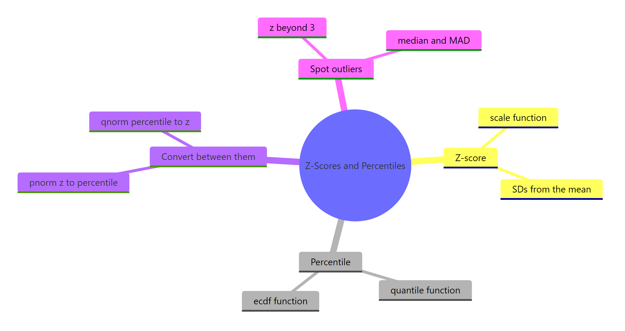
Figure 3: The four things this tutorial covered, at a glance.
| Task | Function | Note |
|---|---|---|
| Standardize a value or column | scale() |
Returns a matrix, wrap in as.numeric(); uses sample SD |
| Value at a percentile | quantile() |
Default type 7 interpolates between points |
| Percentile of a value | ecdf() |
Counts positions, assumes nothing about shape |
| Z-score to percentile | pnorm() |
Assumes a normal distribution |
| Percentile to z-score | qnorm() |
The inverse of pnorm() |
| Robust outlier check | median() and mad() |
Survives extreme values that fool the standard rule |
The one habit that separates a careful analyst from a careless one: reach for empirical percentiles (ecdf() and quantile()) by default, and only convert z-scores to percentiles with pnorm() after you have checked that the data is roughly normal.
References
- R Core Team. stats::scale documentation. Link
- R Core Team. stats::quantile documentation (sample quantile types). Link
- R Core Team. stats::ecdf documentation. Link
- R Core Team. Normal distribution functions (pnorm, qnorm). Link
- R Core Team. stats::mad documentation (median absolute deviation). Link
- Hyndman, R. J. and Fan, Y. (1996). Sample Quantiles in Statistical Packages. The American Statistician, 50(4), 361-365. Link
- Diez, D., Barr, C., and Cetinkaya-Rundel, M. OpenIntro Statistics, 4th Edition (z-scores and the normal model). Link
Continue Learning
- Mean vs Median, SD vs IQR: the mean and standard deviation are the exact ingredients a z-score divides by, so this is the natural prerequisite.
- Normal, t, F and Chi-Squared Distributions in R: a deeper look at the bell curve that
pnorm()andqnorm()are built on. - Sampling Distributions in R: where standardizing leads next, turning z-scores into the foundation of statistical inference.