How Statistical Inference Works (No Formulas Yet)
Statistical inference is how you use a small, manageable sample of data to make a confident, measured guess about a much larger group you could never fully measure. This guide builds the whole idea from the ground up, with no formulas, using simulations you run yourself.
We will use base R for everything except two plots (which use ggplot2), and we will lean on one friendly trick: we will build a pretend world where we secretly know the true answer. That way, every time we make a guess from a sample, we can grade it against the truth and watch how inference actually behaves.
What is statistical inference, in plain English?
Imagine a cook with a huge pot of soup. To judge whether the whole pot is seasoned right, the cook does not drink all of it. They give it one good stir, taste a single spoonful, and decide. That leap, from one spoonful to a verdict about the entire pot, is statistical inference.
In data terms, the pot is the population, everyone or everything you actually care about. The spoonful is the sample, the small part you can afford to look at. The true seasoning of the whole pot is a parameter, the real number you wish you knew. The seasoning you taste in your spoonful is a statistic, the number you actually measure. Inference is the art of using the statistic (the spoonful) to say something trustworthy about the parameter (the pot).
Let us watch the leap happen. We will build a whole city of 100,000 coffee drinkers, where each person drinks some number of cups per week. Because we are building this world, we get to peek at the true city-wide average, something you can almost never do in real life. Then we will pretend we are a market researcher who can only afford to ask 50 people, and see how close our sample guess lands.
Here is what just happened. We created a population of 100,000 numbers whose true average is 8.0 cups. We then drew 50 of those people at random and averaged only them. Our sample of 50 guessed 7.8 cups, without ever looking at the other 99,950 people.

Figure 1: Statistical inference is the leap from a random sample to a measured guess about the whole population.
That gap between 8.0 and 7.8 is the entire subject in miniature. In the real world we would only ever see the 7.8. The 8.0 would stay hidden, which is exactly why we needed to invent a world where we can see both. Let us measure the miss directly.
Our guess was off by two-tenths of a cup, a tiny amount. Fifty people out of a hundred thousand, and we nearly nailed the city average. That reliability is what makes surveys, polls, medical trials, and A/B tests possible. You do not need the whole pot; a good spoonful will do.
Try it: Ask an even smaller group. Take a random sample of just 10 people from the city and see how close their average lands to the true 8 cups.
Click to reveal solution
Explanation: Even 10 people land in the right neighborhood, near 8. A smaller sample is allowed to miss by more, which is a hint about what is coming next.
Why not just measure everyone?
The honest answer is that you usually cannot. A national population is too large to interview. A blood test that used all of your blood would defeat its own purpose. Asking every possible customer would cost more than the decision is worth. So we sample out of pure necessity.
The good news is that we do not need everyone. A single well-stirred spoonful genuinely represents the pot. The catch is in the word stirred. If you only taste the thick stuff that settled at the bottom, your spoonful lies about the whole pot. In sampling, the equivalent of a good stir is picking people at random, so that every person has a fair chance of being chosen.
To feel why this matters, let us run two surveys of the same city. The first is lazy: it only asks the 50 heaviest coffee drinkers, the easy-to-find superfans. The second is fair: it picks 50 people completely at random.
Look at how badly the lazy survey fails. It guessed 19.68 cups when the truth is 8.00, more than double. It was not unlucky; it was rigged from the start by only looking at extreme drinkers. The fair survey, using the same 50-person budget, landed at 7.32, close to the truth. The only difference was randomness in who got picked.
Try it: Bias can tilt the other way too. Build a lazy survey from the 50 lightest drinkers instead and see how wrong it gets.
Click to reveal solution
Explanation: Cherry-picking the lightest drinkers is just as misleading as cherry-picking the heaviest, only in the opposite direction. Bias, not sample size, is what wrecks the guess.
Why does every sample give a different answer?
If two friends each dip their own spoon into the same pot, they taste slightly different things. Neither is wrong; a spoonful is just a little bit random. The same is true of samples. Ask 50 random people today and 50 different random people tomorrow, and you will get two different averages. This bouncing around has a name: sampling variability.
Instead of taking one sample, let us take five thousand. Each one is 50 random people, and each produces its own guess about the city average. We will collect all five thousand guesses in one go and peek at the first eight.
The replicate() function simply repeats the "draw 50 people and average them" experiment 5,000 times and stores each answer. The first eight guesses range from 7.48 to 8.90. They are all in the same ballpark, clustered around 8, but no two are identical. That scatter is the sampling variability made visible.
Now let us look at all 5,000 guesses at once by measuring their spread: the smallest, the largest, and the typical distance from the middle.
Across 5,000 tries, the guesses never fell below 6.64 or rose above 9.74, and a typical guess sat about 0.41 cups away from the center. So a single sample of 50 is not a precise instrument, but it is a reliable one: it lands near the truth, give or take about half a cup. A picture makes this unmistakable.
When you run that block, you see a tidy bell-shaped hill of guesses, tallest right over the true value marked by the vertical line and thinning out on both sides. That pile has a formal name, the sampling distribution, but the picture is the point: the guesses are not scattered randomly, they form a predictable shape centered on the truth.
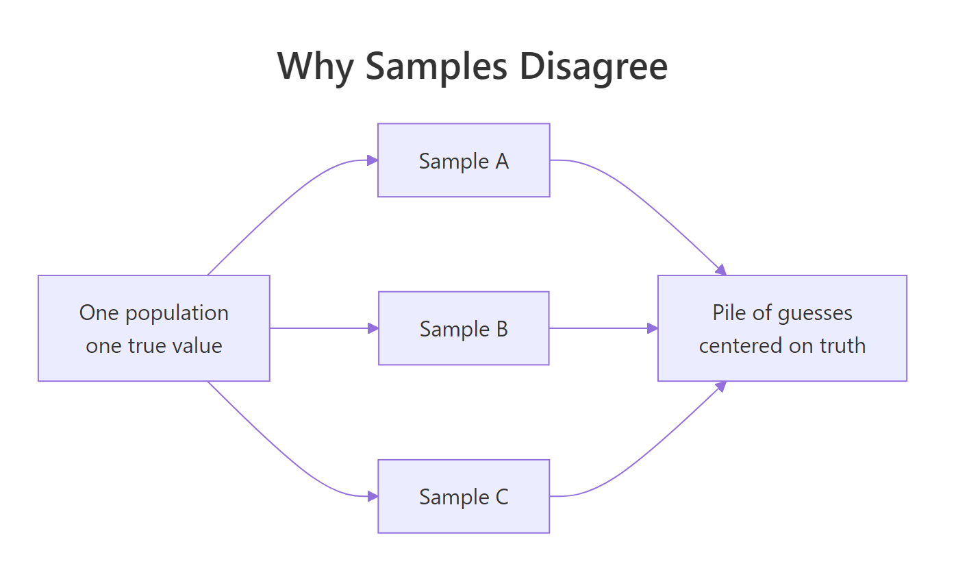
Figure 2: Different samples from the same population give different guesses that pile up around the truth.
Try it: Bigger spoonfuls should wobble less. Repeat the experiment with samples of 200 people instead of 50 and measure the new spread.
Click to reveal solution
Explanation: Quadrupling the sample from 50 to 200 roughly halves the spread, from about 0.41 to about 0.2. That relationship is exactly what the next section is about.
How does a bigger sample make you more sure?
A bigger spoonful is a better miniature of the pot. Ask more people and their average clings more tightly to the truth, because one unusual person gets diluted by all the ordinary ones around them. We just saw a hint of this; now let us map it properly across four sample sizes.
For each size, we repeat the "draw a sample and average it" experiment two thousand times and record how much those guesses typically miss by. That typical miss is just the spread of the guesses we have been measuring all along.
Read down the table and the pattern jumps out. At 25 people a guess typically misses by about 0.57 cups; at 400 people it misses by only about 0.14. More data means less wobble, exactly as intuition promised.
But notice the shape of the improvement. Going from 25 to 100 (four times the data) cut the miss roughly in half, from 0.57 to 0.28. Going from 100 to 400 (four times again) halved it once more, from 0.28 to 0.14. To double your precision, you need about four times the sample, not twice. Accuracy gets expensive.
Try it: Push the sample size higher still. Reuse the spread_at() helper to find the typical miss for a sample of 1,000 people.
Click to reveal solution
Explanation: The wobble keeps shrinking as the sample grows, but ever more slowly. Each extra person helps a little less than the one before.
How do we put a number on our uncertainty?
Reporting a single number like "about 8 cups" hides something important: how sure are we? A far more honest report is a range plus a confidence level, such as "somewhere between 7.4 and 8.5, and we are quite sure." The beautiful part is that this range comes straight from the wobble we have already measured. We are not adding new machinery, just reading what the sampling distribution already told us.
Let us make the range concrete. We will take five thousand guesses from samples of 100 people, then find the band that holds the middle 95% of them, cutting off the lowest 2.5% and the highest 2.5%.
This says that 95% of all possible samples of 100 people produce a guess between 7.44 and 8.54 cups. The true value, 8, sits comfortably inside. So if someone hands you one sample of 100, you can expect its guess to land in that band almost every time.
In real life, though, you only get one sample, and you do not know the truth, so you cannot compute that band directly. Instead you use the typical wobble to build a range around your single guess. Let us first measure that wobble for samples of 100.
A guess from 100 people typically bounces about 0.28 cups. A handy rule is to reach out about two typical-misses on each side of your guess, which covers roughly 95% of the bounce. Now the real test: if every researcher builds such a range around their own single guess, how many of those ranges actually capture the hidden truth? Let us build 100 of them and count.
Ninety-five out of a hundred. Each range was built from its own single sample, blind to the truth, yet 95 of them successfully bracketed the real answer of 8. That number is not a coincidence; it is what "95%" means. Let us see all 100 ranges at once.
The plot shows 100 horizontal ranges, each with its guess marked as a dot, and one vertical line at the true value. Almost all of the ranges cross that line. A handful, about five, miss it entirely and are colored red. Those unlucky few came from samples that happened to land far from the truth.
Try it: A bigger sample should give a narrower band. Build the middle-95% band from guesses of 400 people and compare it to the size-100 band of 7.44 to 8.54.
Click to reveal solution
Explanation: The band shrank from a width of about 1.1 cups (7.44 to 8.54) to about 0.55 cups (7.72 to 8.27). A bigger sample buys a more precise, more useful statement about the truth.
What are the two big jobs of inference?
Now that you understand the wobble and the range, here is the payoff: almost everything statistical inference does is one of just two jobs. The first is estimation: pinning down what a value is, reported as a number plus a range. The second is hypothesis testing: deciding whether a specific claim or difference is real, or whether it is just the wobble playing tricks.
Let us do the estimation job first, using our fair sample of 50 people from earlier. We build a best guess and wrap a range around it using the typical wobble at that size.
Our estimate is 7.32 cups, and our range runs from 6.54 to 8.10. That is the estimation job done: a value and an honest range around it. Now the testing job turns out to be the same range, read differently. Suppose three people each make a claim about the true city average: one says 8, one says 9, one says 10. Which claims can our sample rule out?
The claim of 8 falls inside our range, so our sample cannot rule it out; it is plausible. The claims of 9 and 10 fall outside the range, so this sample gives us grounds to doubt them. That, in one small table, is the seed of every hypothesis test you will ever run: compare a claim against the range of what your data could plausibly produce.
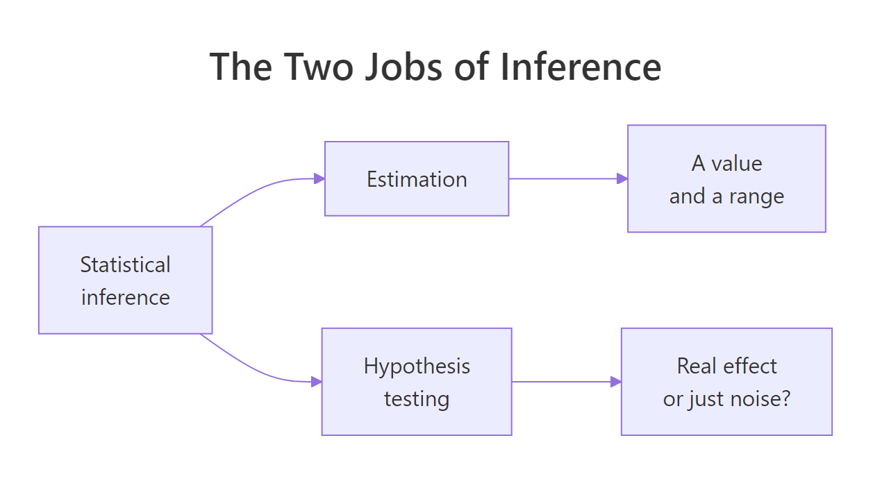
Figure 3: Every inference task is either estimation or hypothesis testing.
Try it: Test one more claim. Using the same range, check whether 7 could be the true city average.
Click to reveal solution
Explanation: 7 sits inside the range, so on this evidence we cannot rule it out. A value like 5 would fall outside and could be ruled out. Your data narrows the field of believable answers rather than picking exactly one.
The Complete Picture: Inference From Start to Finish
So far we invented our population. Let us prove the same logic works on a real dataset by treating R's built-in iris flowers as a population. We will hide from ourselves that we know all 150 flowers, sample just 20 of them, and run the full pipeline: estimate, range, and a check against the truth.
Follow the story in the output. The true average sepal length across all 150 flowers is 5.84 cm, but we only allowed ourselves to see 20 flowers. From those 20 we estimated 5.89 cm, then built a range from 5.55 to 6.23. The truth of 5.84 sits inside our range. We used a sample to make a measured, honest statement about a population, and it worked, with no formulas anywhere in sight.
That is the complete arc of statistical inference: sample fairly, make a guess, quantify the wobble, wrap the guess in a range, and state your confidence in the method. Every advanced technique you will meet later is a more precise version of these same five moves.
Practice Exercises
These combine several ideas from the guide. Each uses fresh variable names so it will not disturb the city and true_average values from earlier. Try each before opening the solution.
Exercise 1: Grade your own guess
Draw a random sample of 30 people from the city population, estimate the true average from it, and check whether your estimate lands within 0.5 cups of the true value. Use set.seed(500) so your answer matches.
Click to reveal solution
Explanation: A sample of 30 guessed 8.17, missing the truth by only 0.17 cups, comfortably inside half a cup. Small samples can still be close; they just carry more wobble than large ones.
Exercise 2: Show that bigger samples wobble less
Measure the typical miss for samples of 20 and compare it to samples of 200, using 2,000 repeats each. Use set.seed(600). Which size wobbles less, and by roughly how much?
Click to reveal solution
Explanation: Samples of 200 wobble about a third as much as samples of 20. Ten times the data cut the typical miss by roughly three times, another view of the "four times the sample to double precision" rule.
Exercise 3: Build a range and test it
Build a 95%-style range for a fresh sample of 80 people (use set.seed(700) for the wobble and set.seed(701) for the sample), then check whether it captures the true average. In one sentence, explain what would happen if you repeated this for many samples.
Click to reveal solution
Explanation: This range runs from 7.20 to 8.47 and captures the true 8.00. If you repeated the whole procedure for many fresh samples, about 95% of the ranges you built would capture the truth, which is exactly what a 95% confidence level promises.
Frequently Asked Questions
Is statistical inference the same as descriptive statistics?
No. Descriptive statistics summarize the data you actually have, such as the average of the 50 people you surveyed. Statistical inference uses that sample to make a measured claim about a larger population you did not measure, and it always comes with a statement of how uncertain that claim is.
Does a 95% range mean there is a 95% chance the true value is inside it?
No, and this is the most common misunderstanding. The 95% describes the method: if you repeated the whole sample-and-build-a-range procedure many times, about 95% of the ranges would contain the truth. Your one particular range either contains the truth or it does not, so the 95% is the long-run hit rate of the recipe, not a probability about your single range.
How big does my sample need to be?
It depends on how precise you need to be. Because the wobble shrinks with the square root of the sample size, you need roughly four times the data to cut your uncertainty in half. Past a point the extra precision is not worth the cost, which is why most polls stop at a few thousand people. See sample size planning for how to choose a number.
Can a bigger sample fix a biased one?
No. Bias is a systematic error in who gets picked, so drawing more people with the same flawed method just gives you a more confident wrong answer. The fix is a fair, random selection, not a larger one.
What is the difference between a parameter and a statistic?
A parameter is the true value in the whole population, like the real city-wide average of 8 cups, and it is usually hidden from you. A statistic is the value you compute from your sample, like the 7.8 cups your 50 people averaged. Inference is the work of using the statistic to say something trustworthy about the parameter.
Summary
Statistical inference is the disciplined leap from a small sample to a confident statement about a large population. You never need the whole pot; a fair spoonful, honestly measured, is enough. Here are the ideas to carry forward.
| Idea | Plain meaning |
|---|---|
| Population vs sample | The whole group you care about, versus the small part you actually measure. |
| Parameter vs statistic | The true value you want (hidden), versus the value your sample gives (seen). |
| Random sampling | The fair "stir" that makes a sample resemble the population; bias cannot be fixed by size. |
| Sampling variability | Every sample gives a slightly different guess; the guesses form a bell centered on the truth. |
| Sample size | More data means less wobble, but you need about four times the sample to double precision. |
| The range and 95% | Report a guess plus a range; "95% confident" describes the method's long-run hit rate, not one range. |
| The two jobs | Estimation finds a value with a range; hypothesis testing checks whether a claim fits that range. |
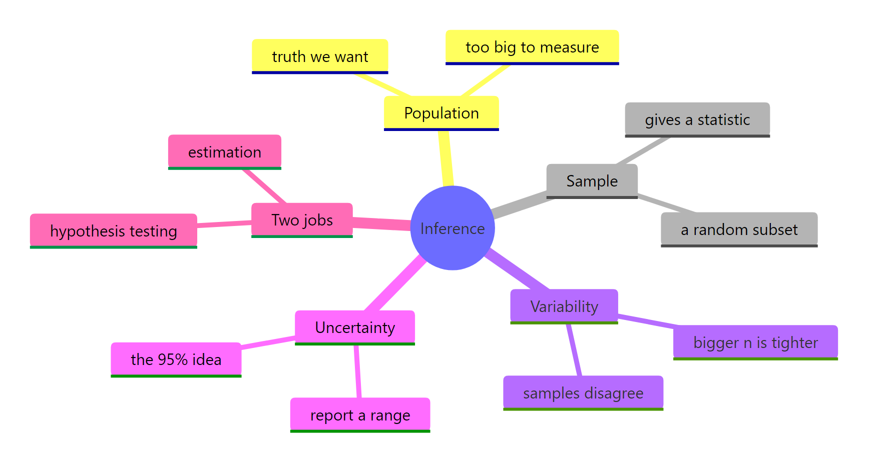
Figure 4: The whole logic of statistical inference on one page.
You now understand the engine behind confidence intervals, hypothesis tests, A/B tests, and polls, all without a single formula. When you meet the formulas later, they will simply be a faster way to compute the ranges and the surprise you just simulated by hand.
References
- Kass, R. E. Statistical Inference: The Big Picture. Statistical Science, 26(1), 2011. Link
- Diez, D., Barr, C., Cetinkaya-Rundel, M. OpenIntro Statistics, 4th Edition. Foundations for inference. Link
- Wasserman, L. All of Statistics: A Concise Course in Statistical Inference. Springer (2004). Link
- R Core Team. An Introduction to R, sampling and simulation. Link
- Wikipedia. Statistical inference. Link
- Frost, J. Statistical Inference: Definition, Methods & Example. Statistics By Jim. Link
Continue Learning
- Central Limit Theorem in R explains why the pile of sample guesses always turns out bell-shaped, the fact that makes ranges work.
- Confidence Intervals in R is the formal, one-sample version of the range you built by simulation here.
- Hypothesis Testing in R turns the "real or just wobble?" question into a precise, repeatable procedure.