GEE vs Mixed Models in R
GEE and mixed models both fix the same problem: data where the rows are not independent, like several measurements on the same person. They part ways on what a coefficient means. A mixed model reports subject-specific effects and how much subjects differ; a generalized estimating equations (GEE) model reports one population-average effect with standard errors that stay valid even if you guess the correlation wrong. This guide builds both ideas from scratch, fits the same data both ways, and shows exactly why their numbers can disagree. It uses base R plus lme4, which run right here in your browser, and shows the GEE fits with geepack to run in your own R session.
What problem do GEE and mixed models both solve?
Ordinary regression assumes every row is an independent draw. That assumption breaks the moment your data has structure: four blood-pressure readings from the same patient, test scores from pupils in the same classroom, or daily sales from the same store. Readings from one patient look more alike than readings from different patients, and pretending otherwise distorts your standard errors. GEE and mixed models are the two standard cures. Let's meet a dataset with exactly this structure and fit our first model.
We will use sleepstudy, which ships with lme4. It records the average Reaction time (in milliseconds) of 18 subjects across 10 days of restricted sleep. Each subject contributes 10 rows, so the rows come in clusters of one person. Here is a mixed model that estimates how reaction time changes per sleepless day.
That one number, 10.47, is the payoff: on average, reaction time slows by about 10.5 milliseconds for each additional day of sleep restriction. The (Days | Subject) part told the model that each subject can have their own starting reaction time and their own slope. Before we unpack what that means, let's look at the raw data so the model feels concrete.
Each row is one subject on one day. Subject 308 appears ten times (days 0 through 9), then subject 309 takes over, and so on. Those ten rows per subject are the correlated cluster. There are 18 subjects and 180 rows in total. To see why ignoring that structure is dangerous, let's fit a plain lm() that treats all 180 rows as independent and compare its standard error for Days to the mixed model's.
Both approaches agree the slope is about 10.467. But the naive model claims a standard error of 1.238, while the mixed model, which knows the readings come in clusters, reports a wider 1.546. The naive model is overconfident: it counted 180 independent facts when it really had 18 people measured repeatedly. Correlated data does not usually change your point estimate by much, but it can badly distort the uncertainty around it, and uncertainty is what your p-values and confidence intervals are built from.
Both GEE and mixed models exist to get that uncertainty right on clustered data. The difference between them, which is the whole point of this guide, is what they hand you in return.
Try it: Fit a simpler mixed model that gives each subject only their own starting point (a random intercept) but a shared slope, written (1 | Subject). Read off the Days fixed effect.
Click to reveal solution
Explanation: The population-level slope is still about 10.47. Changing the random-effects structure mainly changes how the model accounts for correlation and uncertainty, not the average trend itself.
What does each model actually estimate?
Here is the fork in the road. A mixed model and a GEE model can be handed the identical dataset and the identical formula, yet they answer two different questions. A mixed model answers a conditional, subject-specific question: "for a given subject, how does the outcome change?" A GEE model answers a marginal, population-average question: "averaged across the whole population, how does the average outcome change?" Understanding this split is the key to everything else.
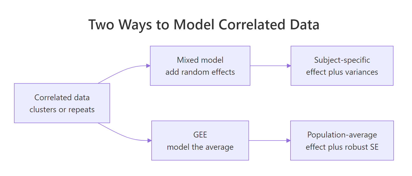
Figure 1: Two routes for correlated data: add random effects (mixed) or model the average directly (GEE).
The mixed model builds the correlation from the inside out. It says each subject $i$ carries a personal offset $b_i$, drawn from a distribution, and models the outcome given that offset. In symbols, writing $g$ for the link function (the transformation the model applies to the mean: the identity for a plain linear model, the log-odds for a logistic one), subject $i$, and measurement $j$:
$$g\big(E[Y_{ij} \mid b_i]\big) = \beta_0 + \beta_1 x_{ij} + b_i$$
The GEE model never introduces $b_i$ at all. It models the average outcome directly, having already averaged over every subject:
$$g\big(E[Y_{ij}]\big) = \beta_0 + \beta_1 x_{ij}$$
Where in both, $Y_{ij}$ is the outcome for subject $i$ at measurement $j$, $x_{ij}$ is the predictor, and $b_i$ is subject $i$'s random effect. The mixed model's $\beta_1$ is a within-subject effect; the GEE model's $\beta_1$ is a between-population average.
Because the mixed model estimates those $b_i$ offsets, it can report things GEE cannot. First, how much subjects differ from each other, as variance components.
Read this as three sources of spread. Subjects differ in their baseline reaction time with a standard deviation of about 24.7 ms, they differ in their day-to-day slope with a standard deviation of about 5.9 ms, and after accounting for those, the leftover noise has a standard deviation of about 25.6 ms. GEE hands you none of these numbers, because it never modeled individual subjects. Second, the mixed model can estimate each subject's personal deviation.
Subject 309 starts about 40 ms faster than average and their slope is 8.6 ms shallower than the population slope. That is a subject-specific story. Now let's fit the same sleepstudy data with GEE and see what it reports instead. The GEE engine here is geepack, which is not part of the in-browser runtime, so run this block in your own R session.
# install.packages("geepack") if you do not have it
library(geepack)
g_lin <- geeglm(Reaction ~ Days, id = Subject, data = sleepstudy,
                family = gaussian, corstr = "exchangeable")
round(coef(g_lin), 2)
#> (Intercept)        Days
#>      251.41       10.47
round(summary(g_lin)$coefficients[, 1:2], 3)
#>             Estimate Std.err
#> (Intercept)  251.405   6.632
#> Days          10.467   1.502
The GEE slope for Days is 10.47, the same as the mixed model, with a robust standard error of 1.502. Notice what is missing: no variance components, no per-subject offsets. GEE gives you the population-average line and valid standard errors, and stops there. On this dataset the two methods produce the same slope, which raises a fair question: if they agree, why does anyone care about the distinction? The answer is that they agree here because reaction time is modeled on its natural scale with an identity link. As soon as the link becomes nonlinear, the agreement collapses.
Try it: The intraclass correlation (ICC) summarizes how much of the total variation is between subjects. From a random-intercept model, it is the between-subject variance divided by the total variance. Compute it for sleepstudy.
Click to reveal solution
Explanation: About 0.589 of the total variation in reaction time sits between subjects rather than within them. A high ICC means the clustering is strong, which is exactly when respecting it matters most.
Why do the coefficients differ on binary data?
For a yes/no outcome you use a logistic link, and the link is an S-shaped curve, not a straight line. Averaging a bundle of S-curves that each sit at a different height does not give back the same S-curve; it gives a flatter one. That flattening is why the population-average slope from GEE comes out smaller in magnitude than the subject-specific slope from a mixed model. Let's build a dataset where we know the true subject-specific effect, then watch the two methods disagree.
We will simulate 250 subjects, each measured 6 times, with a treatment indicator x. We bake in a true subject-specific slope of 1.0 on the log-odds scale, plus a subject random intercept with a standard deviation of 1.5.
In that last step, plogis() turns each subject's log-odds (eta) into a probability, and rbinom() draws the 0 or 1 outcome from that probability. Now fit a mixed logistic model with glmer(). Because we built the data with a subject-specific effect, this is the method aimed at the scale we generated, and it should land near the true value of 1.0.
The conditional (subject-specific) slope is 0.860, close to the true 1.0 given sampling noise. Its odds ratio is $e^{0.86} \approx 2.36$: for a given subject, treatment multiplies the odds of a positive outcome by about 2.4. Now fit the population-average version with GEE on the identical data. Run this in your own R session.
library(geepack)
g_bin <- geeglm(y ~ x, id = subj, data = bin, family = binomial,
                corstr = "exchangeable")
round(summary(g_bin)$coefficients[, 1:2], 3)
#>             Estimate Std.err
#> (Intercept)   -0.328   0.090
#> x              0.640   0.092
The GEE slope is 0.640, clearly smaller than the mixed model's 0.860. Its odds ratio is $e^{0.64} \approx 1.90$: averaged across the whole population, treatment multiplies the odds by about 1.9. Both models are correct. They simply answer different questions, and on a nonlinear scale the two answers are genuinely different numbers. There is even a well-known approximation linking them:
$$\beta^{\text{PA}} \approx \frac{\beta^{\text{SS}}}{\sqrt{1 + 0.346\,\sigma_b^2}}$$
Where $\beta^{\text{PA}}$ is the population-average coefficient GEE targets, $\beta^{\text{SS}}$ is the subject-specific coefficient the mixed model targets, $\sigma_b^2$ is the variance of the subject random intercepts, and 0.346 is a constant from the logistic approximation. Let's plug in the numbers our mixed model estimated and see if the approximation lands near the GEE result.
The formula turns the conditional 0.860 into a predicted marginal 0.684, in the same neighborhood as the GEE estimate of 0.640. The mechanism is real: the more subjects vary (the larger $\sigma_b$), the more the population-average effect shrinks toward zero relative to the subject-specific one.
Try it: Convert a conditional log-odds coefficient into an odds ratio. Use the mixed model's slope of 0.86.
Click to reveal solution
Explanation: Exponentiating a log-odds coefficient gives an odds ratio. Here the subject-specific odds ratio is 2.36, larger than the population-average 1.90 we saw from GEE, exactly the gap the approximation predicts.
How does each handle the correlation itself?
Both methods have to say something about how measurements within a cluster relate, but they do it in opposite ways. A mixed model handles correlation implicitly: once you specify the random effects, the within-subject correlation is a consequence of the model, estimated by maximum likelihood. A GEE model handles correlation explicitly: you pick a working correlation structure as a separate ingredient, and GEE uses it only to improve efficiency. Crucially, GEE then wraps the result in robust (sandwich) standard errors, so your inference stays valid even if the working structure you picked is wrong.
You choose the GEE working structure with the corstr argument. Here are the common options.
| Working correlation | What it assumes | Use when |
|---|---|---|
independence |
No within-cluster correlation | A baseline, or when robust SEs do all the work |
exchangeable |
Every pair in a cluster is equally correlated | Clusters with no natural order (people in a household) |
ar1 |
Correlation fades as observations get further apart | Evenly spaced time points |
unstructured |
A separate correlation for every pair | Few time points and plenty of clusters |
Let's confirm the robustness claim on the binary data. We fit GEE with two different working structures and check that the treatment estimate barely moves. Run this locally.
library(geepack)
g_ex <- geeglm(y ~ x, id = subj, data = bin, family = binomial, corstr = "exchangeable")
g_ar <- geeglm(y ~ x, id = subj, data = bin, family = binomial, corstr = "ar1")
c(exchangeable = round(coef(g_ex)[["x"]], 3),
  ar1          = round(coef(g_ar)[["x"]], 3))
#> exchangeable          ar1
#>        0.640        0.655
The slope is 0.640 under exchangeable and 0.655 under AR-1: essentially the same conclusion despite a different assumption about the correlation. That stability is the practical appeal of GEE. You do not have to get the correlation structure exactly right, because the robust standard errors correct for the mismatch. The mixed model, by contrast, encodes the correlation through its random effects, and you can read that structure back out of the fitted model.
The Corr column, 0.066, is the estimated correlation between a subject's random intercept and their random slope. The mixed model did not treat correlation as a nuisance to be robustly ignored; it estimated it as a meaningful part of the story. That difference in philosophy has a catch, though.
Try it: The two mixed models we fit differ in flexibility: a random intercept only, versus random intercept plus slope. Compare them with AIC(), where a lower value indicates a better trade-off of fit and complexity.
Click to reveal solution
Explanation: The random-slope model has the lower AIC (1755.6 vs 1794.5), so the data support letting each subject have their own slope. This kind of likelihood-based model comparison is available for mixed models but not for GEE, which has no full likelihood.
What assumptions does each make about missing data?
Real longitudinal data is rarely complete: patients miss visits, subjects drop out. The two methods make different promises about when missing data is safe, and the difference can decide which one you trust. In brief, a standard GEE is valid when data are missing completely at random (MCAR), meaning missingness is unrelated to anything. Likelihood-based mixed models make the weaker, more realistic assumption of missing at random (MAR), meaning missingness can depend on observed data. That makes mixed models more forgiving of the dropout patterns you actually see in practice.
Let's demonstrate the easy case first: data punched out completely at random. We copy sleepstudy, blank out 30 reaction times at random, and refit the mixed model.
With 150 of the original 180 rows remaining, the slope is still about 10.0, close to the 10.47 from the full data. Under MCAR, both GEE and mixed models stay unbiased. The gap opens under MAR, for example when subjects who are getting worse drop out. There, a likelihood-based mixed model still recovers the right answer using the observed measurements, while a plain GEE would need inverse-probability weights to fix the bias. Here is the fuller comparison.
| Property | Mixed model (lme4) |
GEE (geepack) |
|---|---|---|
| Estimand | Subject-specific (conditional) | Population-average (marginal) |
| Correlation | Modeled via random effects | Working structure plus robust SE |
| Estimation | Maximum likelihood | Quasi-likelihood, no full likelihood |
| Extra output | Variance components, per-subject effects | Robust SEs only |
| Missing data valid under | MAR | MCAR (or MAR with weights) |
| Model comparison | AIC, likelihood-ratio tests | QIC (no likelihood-ratio test) |
Try it: Confirm the missingness is spread across subjects rather than wiping out whole people. Count how many complete reaction times each subject still has, using tapply().
Click to reveal solution
Explanation: Each subject keeps 8 or 9 of their 10 records, so no subject is lost entirely. That even spread is what "completely at random" looks like, and it is the friendly case for both methods.
Which one should you use?
The decision is not about which method is better; it is about which question you are asking. Trace your goal through the map below and the choice makes itself.
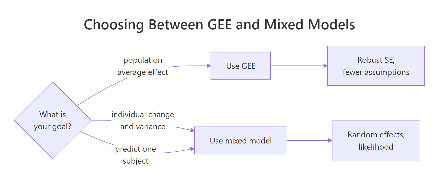
Figure 2: Pick the method from the question you are answering.
Choose GEE when you want the population-average effect and nothing more: the average change a public-health official or policy maker cares about, stated with robust standard errors and few assumptions. It shines for marginal questions on binary or count outcomes, and it is happy with many clusters and simple within-cluster structure. See the deep dive on GEE for correlated categorical data for the full geepack workflow.
Choose a mixed model when you care about individuals: how much subjects differ, how a specific subject is likely to respond, or a variance decomposition of where the noise lives. It is also the model for complex designs (nested or crossed groups) and for likelihood-based comparisons and MAR missing data. The companion guide on random intercepts and slopes walks through building these models step by step.
| Your goal | Reach for |
|---|---|
| The average effect across a population | GEE |
| How much individuals vary | Mixed model |
| A prediction for one specific subject | Mixed model |
| Binary or count outcome, marginal question, many clusters | GEE |
| Nested or crossed grouping structure | Mixed model |
| Robust inference with a possibly-wrong correlation guess | GEE |
Try it: A mixed model can produce both the population line and a single subject's line. The population intercept and slope are fixef(m_mix); subject 308's own line is coef(m_mix)$Subject["308", ]. Print both and compare.
Click to reveal solution
Explanation: The population slope is 10.47, but subject 308's own slope is 19.67, nearly double. A mixed model can tell you both; GEE only ever reports the population line.
Practice Exercises
These combine several ideas from the tutorial. Try each before opening the solution. The exercises use fresh variable names so they will not overwrite the models you fit above.
Exercise 1: Recover a subject-specific effect from binary data
Simulate a small clustered binary dataset (120 subjects, 5 measurements each) with a true subject-specific slope of 0.8, fit glmer(), and report the conditional slope and its odds ratio. Then say in one line why a GEE fit would return a smaller number.
Click to reveal solution
Explanation: The conditional slope is 1.05 (odds ratio 2.85), a bit above the true 0.8 we set but within the sampling noise you expect from a single simulated dataset of this size. A GEE model would average the logistic curves over subjects and return a smaller, flatter population-average slope.
Exercise 2: Name what GEE cannot report
Fit the random-intercept-and-slope model on sleepstudy, print its variance components, and identify the three quantities in that output that a GEE model would never give you.
Click to reveal solution
Explanation: The three quantities GEE cannot report are the between-subject intercept standard deviation (24.74), the between-subject slope standard deviation (5.92), and the correlation between them (0.066). GEE never models individual subjects, so it has no variance components at all.
Exercise 3: Quantify how far one subject sits from the average
Using the mixed model, build the fitted line for subject 308 and the population-average line, then compute the gap in predicted reaction time on Day 9.
Click to reveal solution
Explanation: At Day 9 the population line predicts about 345.6 ms, but subject 308 is predicted at 430.7 ms, a gap of 85 ms. That subject-specific prediction is something only the mixed model can produce; GEE would return only the 345.6 population value.
Frequently Asked Questions
Can a GEE model give me random effects or a prediction for one subject? No. GEE models the population average and never estimates subject-level offsets, so it cannot report variance components or predict a specific subject's trajectory. If you need those, use a mixed model.
If GEE and my mixed model give different coefficients on binary data, is one of them wrong? Neither is wrong. The mixed model reports a subject-specific (conditional) effect and GEE reports a population-average (marginal) effect. On a logistic or log link these are genuinely different quantities, with the subject-specific one always larger in magnitude.
Do I need different packages for each? Yes. In R, lme4 (with lmer() and glmer()) fits mixed models, and geepack (with geeglm()) fits GEE models. The nlme package also fits mixed models and marginal models via generalized least squares.
When the outcome is continuous with an identity link, does the choice matter? For the fixed-effect estimates, much less. Averaging a straight line preserves its slope, so GEE and a linear mixed model report essentially the same coefficient. The mixed model still adds variance components and subject-level prediction on top.
How many clusters do I need for GEE? As a rule of thumb, at least 30 to 40. GEE's robust standard errors rely on a large number of clusters; with few clusters they run too small, and a likelihood-based mixed model or a small-sample correction is safer.
Summary
GEE and mixed models are two valid answers to correlated data, aimed at two different questions. Pick the one whose estimand matches what you actually want to report.
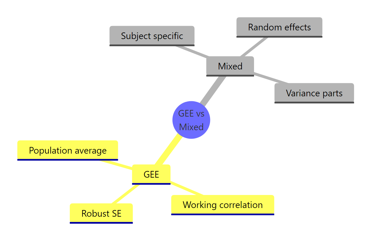
Figure 3: The two model families at a glance.
| Question | Mixed model | GEE |
|---|---|---|
| What does a coefficient mean? | Subject-specific (conditional) | Population-average (marginal) |
| How is correlation handled? | Random effects, by likelihood | Working structure plus robust SE |
| What extra do you get? | Variance components, per-subject effects | Robust standard errors |
| Binary/count coefficient size | Larger in magnitude | Smaller in magnitude |
| Missing data safe under | MAR | MCAR (or MAR with weights) |
| R tool | lme4::lmer / glmer |
geepack::geeglm |
The one sentence to remember: a mixed model tells you about individuals, GEE tells you about the population average, and on a nonlinear scale those are different numbers on purpose.
References
- Halekoh, U., Hojsgaard, S., and Yan, J. (2006). The R Package geepack for Generalized Estimating Equations. Journal of Statistical Software. Link
- Bates, D., Machler, M., Bolker, B., and Walker, S. (2015). Fitting Linear Mixed-Effects Models Using lme4. Journal of Statistical Software. Link
- UVA Library. Getting Started with Generalized Estimating Equations. Link
- Comparing generalized estimating equations and linear mixed effects models for estimating marginal association (2022). PMC. Link
- geepack package on CRAN. Link
- lme4 package on CRAN. Link
- nlme package on CRAN (mixed models and marginal GLS models). Link
Continue Learning
- Random Intercepts and Slopes in R: build mixed models from the ground up, the natural next step for the subject-specific side.
- GEE for Correlated Categorical Data in R: the full geepack workflow for population-average models on binary outcomes.
- Mixed Model Inference in R: p-values, confidence intervals, and bootstrapping for the mixed-model coefficients you fit here.