Multiple Imputation with mice in R
Multiple imputation fills each missing value several times to build several complete datasets, analyzes each one, then pools the answers so your standard errors reflect the uncertainty the missing data really carries. The mice package in R runs this whole workflow with a handful of functions, and this guide walks through every step on a real dataset.
What problem does multiple imputation actually solve?
Almost every real dataset has holes in it. A sensor drops out, a survey question gets skipped, a lab result never comes back. The two reflexes most people reach for, deleting the incomplete rows or filling the blanks with a column average, both quietly bend your results. Before we fix that, let's see the damage with our own eyes.
We will use airquality, a dataset built into R that records daily air-quality readings in New York in 1973. It ships with genuine missing values, so nothing here is staged. Our first job is simply to find the holes.
The dataset has 153 rows and 6 columns. The colSums(is.na(...)) line counts the NA (missing) entries per column: 37 missing Ozone values and 7 missing Solar.R values, with the rest complete. That is a lot of missing ozone for a dataset this size.
The oldest fix is to keep only the rows that are complete, an approach called listwise deletion (also known as complete-case analysis). Let's measure what that costs us.
Dropping every row with any gap throws away 42 of 153 rows, about 27 percent of the data. That waste matters, because smaller samples give wider, less certain estimates. Here is the regression we will return to throughout this guide, fit on the 111 complete rows.
The Temp row says ozone rises about 1.65 units for each extra degree, with a standard error of 0.254. The standard error is our measure of how precise that estimate is: smaller means more certain. Hold onto the value 0.254, because we will watch it change as we try better and worse ways of handling the gaps.
mice package, runs in a local R session rather than in your browser, so those blocks are labelled "run locally". Everything in the browser-runnable blocks works as you read.Try it: Instead of raw counts, show the percentage of values missing in each column. The helper colMeans(is.na(x)) gives the fraction missing per column.
Click to reveal solution
Explanation: is.na() turns each column into TRUE/FALSE, and the mean of TRUE/FALSE values is the fraction that are TRUE. Almost a quarter of the ozone readings are missing.
Why does filling in the mean give you the wrong answer?
The next reflex after deleting rows is to keep them and paste the column average into every blank. It feels harmless, since the mean is a reasonable central guess. The problem is that it pretends every guess is a known fact, and that pretense quietly distorts three things at once: the spread of the data, the relationships between variables, and the honesty of your standard errors.
Start with spread. When you drop the same number into 37 slots, you pile up a spike of identical values at the mean, which shrinks the variability.
The standard deviation of ozone falls from 32.99 to 28.69 the moment we fill the blanks with the mean. The data now looks less variable than it truly is. Relationships suffer too, because those flat, identical fills carry no information about the other columns.
The real correlation between ozone and temperature is 0.698, but after mean-filling it drops to 0.609. We have weakened a real relationship between the two variables. Now the part that matters most for any analysis: what mean imputation does to the regression coefficient you actually care about.
Look at the Temp estimate: it has fallen from 1.65 in the complete-case model to 1.24 here, a drop of about a quarter. The flat imputed points bias the slope toward zero. At the same time the standard error shrank to 0.209, smaller than the complete-case 0.254, so the model reports more confidence in a coefficient that is now further from the truth.
Try it: Repeat the spread check for Solar.R. Mean-fill its 7 missing values and compare the standard deviation before and after.
Click to reveal solution
Explanation: The spread shrinks less here (90.06 to 87.96) because only 7 values were filled, versus 37 for ozone. The more you impute with a flat value, the more damage it does.
How does multiple imputation fix the uncertainty problem?
The trouble with a single filled-in value is that it hides your ignorance. You did not actually see that ozone reading, so any one number you write down is just one guess among many that were plausible. Multiple imputation takes that idea literally: instead of one guess per blank, it makes several, each drawn with a bit of random variation, so the guesses disagree with each other on purpose.
That disagreement is the whole point. If you fill the gaps five different ways and your analysis gives nearly the same answer every time, the missing data barely mattered. If the answer jumps around, the missing data carried real uncertainty, and multiple imputation measures exactly how much. The workflow has three steps, shown below.

Figure 1: The three steps of multiple imputation: impute m times, analyze each dataset, then pool the results into one honest estimate.
We can feel this out with plain R before touching any package. Let's fill the 37 missing ozone values by randomly borrowing real observed ozone readings, then compute the mean. Do that five separate times and watch the answer wobble.
Each of the five fills gives a slightly different mean ozone, from 40.56 to 42.62. None is more correct than the others; they are all consistent with the data we have. The gap between them is information, and we can put a number on it.
That 0.915 is the extra uncertainty single imputation throws away. Statisticians call it the between-imputation variance, and it is precisely the wobble you get from not knowing the true values. Multiple imputation keeps this number and folds it into your final standard errors, which is why its answers stay honest.
Try it: Widen the experiment. Draw 20 filled versions instead of 5 and report the smallest and largest mean you see.
Click to reveal solution
Explanation: Across 20 fills the mean ozone ranges from 39.25 to 43.46. Any single-number answer inside that band was possible, which is why reporting just one hides real uncertainty.
How do you run mice on a real dataset?
Our hand-rolled random fill captured the right idea, but a serious method needs to respect the relationships between columns, not just resample one variable in isolation. That is what the mice package does. The name stands for Multivariate Imputation by Chained Equations, and the plain-English version is this: mice imputes each incomplete column using a small model built from all the other columns, cycling through them until the fills settle down.
Before imputing, it pays to look at the shape of the missingness. The md.pattern() function lays out which combinations of missing values actually occur.
library(mice)
md.pattern(airquality, plot = FALSE)
#>     Wind Temp Month Day Solar.R Ozone
#> 111    1    1     1   1       1     1  0
#> 35     1    1     1   1       1     0  1
#> 5      1    1     1   1       0     1  1
#> 2      1    1     1   1       0     0  2
#>        0    0     0   0       7    37 44
Each row is a pattern, and the leading number counts how many data rows follow it. A 1 means present and a 0 means missing. So 111 rows are fully complete, 35 rows are missing only Ozone, 5 rows are missing only Solar.R, and just 2 rows are missing both. The bottom line totals the missing values per column. Now we impute.
imp <- mice(airquality, m = 5, method = "pmm", seed = 123, printFlag = FALSE)
imp
#> Class: mids
#> Number of multiple imputations:  5
#> Imputation methods:
#>   Ozone Solar.R    Wind    Temp   Month     Day
#>   "pmm"   "pmm"      ""      ""      ""      ""
#> PredictorMatrix:
#>         Ozone Solar.R Wind Temp Month Day
#> Ozone       0       1    1    1     1   1
#> Solar.R     1       0    1    1     1   1
#> Wind        1       1    0    1     1   1
#> Temp        1       1    1    0     1   1
#> Month       1       1    1    1     0   1
#> Day         1       1    1    1     1   0
Two arguments do the heavy lifting. m = 5 asks for five complete datasets, and seed = 123 makes the random draws reproducible so you get these exact numbers. The printout confirms mice used the pmm method for the two incomplete columns and left the complete ones alone.
The pmm label is worth unpacking. It stands for predictive mean matching, and it works by finding a few real rows whose predicted value is closest to the one it needs to fill, then copying an actual observed value from one of them. Because every fill is a value that genuinely occurred in the data, imputed ozone is always a plausible ozone reading, never a negative number or an impossible spike. The PredictorMatrix in the printout above shows which columns feed each imputation model; a 1 means "use this column as a predictor".
Each of the five datasets is now complete. Let's confirm there are no gaps left in the first one.
completed_1 <- complete(imp, 1)
colSums(is.na(completed_1))
#>   Ozone Solar.R    Wind    Temp   Month     Day
#>       0       0       0       0       0       0
Zero missing everywhere. The complete(imp, 1) call pulls out the first filled dataset as an ordinary data frame you could analyze directly. The key is that the five datasets differ in exactly the cells that were missing.
imp$imp$Ozone[1:5, ]
#>     1  2  3  4  5
#> 5  18  1 37 18 32
#> 10 12 30 30 20 20
#> 25 18  8  8 28  6
#> 26 13 18 18 20 13
#> 27 20 11 21 32 20
Each row here is one originally-missing ozone value, and the five columns are the five imputations. Row 5, for example, was filled with 18, 1, 37, 18, and 32 across the five datasets. That spread across the columns is the same uncertainty we measured by hand earlier, now respecting every predictor.
Try it: Pull out the third completed dataset and confirm it has 153 rows and no missing values.
# Goal: use complete(imp, 3), then report its row count and total NAs.
# completed_3 <- complete(imp, 3)
# c(rows = nrow(completed_3), missing = sum(is.na(completed_3)))
Click to reveal solution
completed_3 <- complete(imp, 3)
c(rows = nrow(completed_3), missing = sum(is.na(completed_3)))
#>    rows missing
#>     153       0
Explanation: complete(imp, 3) returns the third of the five imputed datasets, complete and ready for analysis. Every imputation restores all 153 rows.
How do you pool the results with Rubin's rules?
You now have five complete datasets, so the temptation is to pick one and analyze it. Do not. Analyzing a single imputed set throws away the disagreement between the five, which is the very uncertainty we worked to capture. Instead you run your analysis on all five, then combine the answers with a recipe called Rubin's rules. The mice package makes this two lines.
The with() function runs the same model on each imputed dataset, and pool() combines the five sets of coefficients into one.
fit <- with(imp, lm(Ozone ~ Temp + Wind + Solar.R))
pooled <- pool(fit)
ps <- summary(pooled)
data.frame(term = ps$term,
           estimate = round(ps$estimate, 3),
           std.error = round(ps$std.error, 3),
           statistic = round(ps$statistic, 2),
           p.value = round(ps$p.value, 4))
#>          term estimate std.error statistic p.value
#> 1 (Intercept)  -62.907    22.861     -2.75  0.0094
#> 2        Temp    1.618     0.241      6.72  0.0000
#> 3        Wind   -3.075     0.655     -4.70  0.0000
#> 4     Solar.R    0.053     0.026      2.01  0.0595
This is the payoff. The pooled Temp estimate is 1.618, almost identical to the complete-case value of 1.652 and a world away from the mean-imputed 1.241. Multiple imputation recovered the honest slope. Now compare the standard errors side by side, because the story there is subtle.
| Approach | Rows used | Temp estimate |
Temp std. error |
|---|---|---|---|
| Complete-case (drop rows) | 111 | 1.652 | 0.254 |
| Single mean imputation | 153 | 1.241 | 0.209 |
| Multiple imputation | 153 | 1.618 | 0.241 |
The pooled standard error of 0.241 is smaller than the complete-case 0.254, because multiple imputation uses all 153 rows instead of discarding 42, so it recovers real information. Yet it is larger than the mean-imputed 0.209, because it honestly adds back the uncertainty that single imputation pretended away. Multiple imputation is both more efficient and more truthful at the same time.
If you like to see the machinery, Rubin's rules combine the five analyses like this. The intuition is that your total uncertainty has two parts: the ordinary uncertainty inside each analysis, plus the extra uncertainty that comes from the five imputations disagreeing.
$$T = \bar{U} + \left(1 + \frac{1}{m}\right) B$$
Where:
- $T$ is the total variance of the pooled estimate (its squared standard error)
- $\bar{U}$ is the average within-imputation variance, the ordinary uncertainty averaged over the five analyses
- $B$ is the between-imputation variance, how much the estimate itself varied across the five datasets
- $m$ is the number of imputations, here 5
That $B$ term is the piece single imputation drops. The mice package reports how large it is through three diagnostics.
pd <- pooled$pooled
data.frame(term = pd$term,
           riv = round(pd$riv, 3),
           lambda = round(pd$lambda, 3),
           fmi = round(pd$fmi, 3))
#>          term   riv lambda   fmi
#> 1 (Intercept) 0.386  0.278 0.317
#> 2        Temp 0.252  0.201 0.230
#> 3        Wind 0.377  0.274 0.312
#> 4     Solar.R 0.718  0.418 0.473
The most useful column is fmi, the fraction of missing information. It estimates how much of the information about each coefficient was lost to missing data. For Solar.R it is 0.473, meaning nearly half the information behind that coefficient depends on imputed values, so treat it with the most caution. The riv (relative increase in variance) and lambda columns tell the same story from slightly different angles.
Try it: Pool a simpler model that predicts Ozone from Temp alone, and report the pooled coefficients.
# Goal: with(imp, lm(Ozone ~ Temp)), then summary(pool(...)).
# ex_fit <- with(imp, lm(Ozone ~ Temp))
# summary(pool(ex_fit))
Click to reveal solution
ex_fit <- with(imp, lm(Ozone ~ Temp))
ex_ps <- summary(pool(ex_fit))
data.frame(term = ex_ps$term,
           estimate = round(ex_ps$estimate, 3),
           std.error = round(ex_ps$std.error, 3))
#>          term estimate std.error
#> 1 (Intercept) -134.818    16.599
#> 2        Temp    2.275     0.215
Explanation: With Temp as the only predictor, its pooled slope is larger (2.275) because it now absorbs effects that were shared with Wind and Solar.R in the full model. The pooling step is identical no matter which model you fit.
How do you check that the imputations are trustworthy?
Imputation is not magic, so you should verify two things before believing the pooled numbers: that the algorithm settled down, and that the values it invented look like the values you actually observed. Both checks are quick.
First, convergence. Mice fills the columns in cycles, and you want the results to stabilize rather than drift as the cycles go on. The chainMean element stores the mean of the imputed ozone values at each iteration for each of the five chains.
round(imp$chainMean["Ozone", , ], 1)
#>   Chain 1 Chain 2 Chain 3 Chain 4 Chain 5
#> 1    44.3    34.9    40.9    37.8    35.8
#> 2    40.1    42.9    39.8    39.5    42.2
#> 3    39.7    39.4    39.2    46.9    39.6
#> 4    36.3    44.7    40.6    45.1    39.2
#> 5    36.1    44.9    40.0    45.5    48.8
Read down each column: the values bounce around in the low 40s without climbing or falling steadily, and the five chains overlap rather than separating into lanes. That is what healthy convergence looks like. In a local session, plot(imp) draws these same traces as lines, and a clean plot shows tangled, drift-free bands. If you ever see the chains trending or splitting apart, raise the iteration count with the maxit argument.
Second, plausibility. The imputed ozone values should occupy roughly the same range as the observed ones. Let's compare their five-number summaries.
obs_oz <- airquality$Ozone[!is.na(airquality$Ozone)]
imp_oz <- unlist(imp$imp$Ozone)
round(rbind(observed = summary(obs_oz), imputed = summary(imp_oz)), 1)
#>          Min. 1st Qu. Median Mean 3rd Qu. Max.
#> observed    1      18   31.5 42.1    63.2  168
#> imputed     1      20   35.0 43.0    63.0  135
The two rows line up closely. The imputed median (35.0) and mean (43.0) sit right beside the observed median (31.5) and mean (42.1), and both span a similar range. The picture below makes the overlap visual, plotting the density of observed ozone against the density of the imputed values.
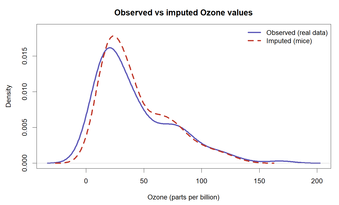
Figure 2: Imputed Ozone values (dashed) follow the shape of the observed values (solid), a sign the imputation model is behaving.
The dashed imputed curve traces the solid observed curve, including the long right tail of high-ozone days. In a local session, densityplot(imp) and stripplot(imp) produce polished versions of this check for every imputed column at once.
Try it: Compare the standard deviation of the observed ozone with the standard deviation of the imputed ozone. They should be close, unlike the shrunken mean-imputation spread from earlier.
# Goal: sd of obs_oz vs sd of imp_oz (both defined above).
# c(observed_sd = sd(obs_oz), imputed_sd = sd(imp_oz))
Click to reveal solution
c(observed_sd = round(sd(obs_oz), 1), imputed_sd = round(sd(imp_oz), 1))
#> observed_sd  imputed_sd
#>        33.0        28.9
Explanation: The imputed spread (28.9) is a little narrower than the observed (33.0), which is expected because imputations pull slightly toward the center, but it is far healthier than the flat mean-fill that collapsed the spread to a spike.
When can you trust multiple imputation? (MCAR, MAR, MNAR)
Multiple imputation is powerful, but it rests on an assumption about why the data is missing in the first place. Statisticians sort the reasons into three mechanisms, and knowing which one you face tells you whether imputation will give an honest answer.
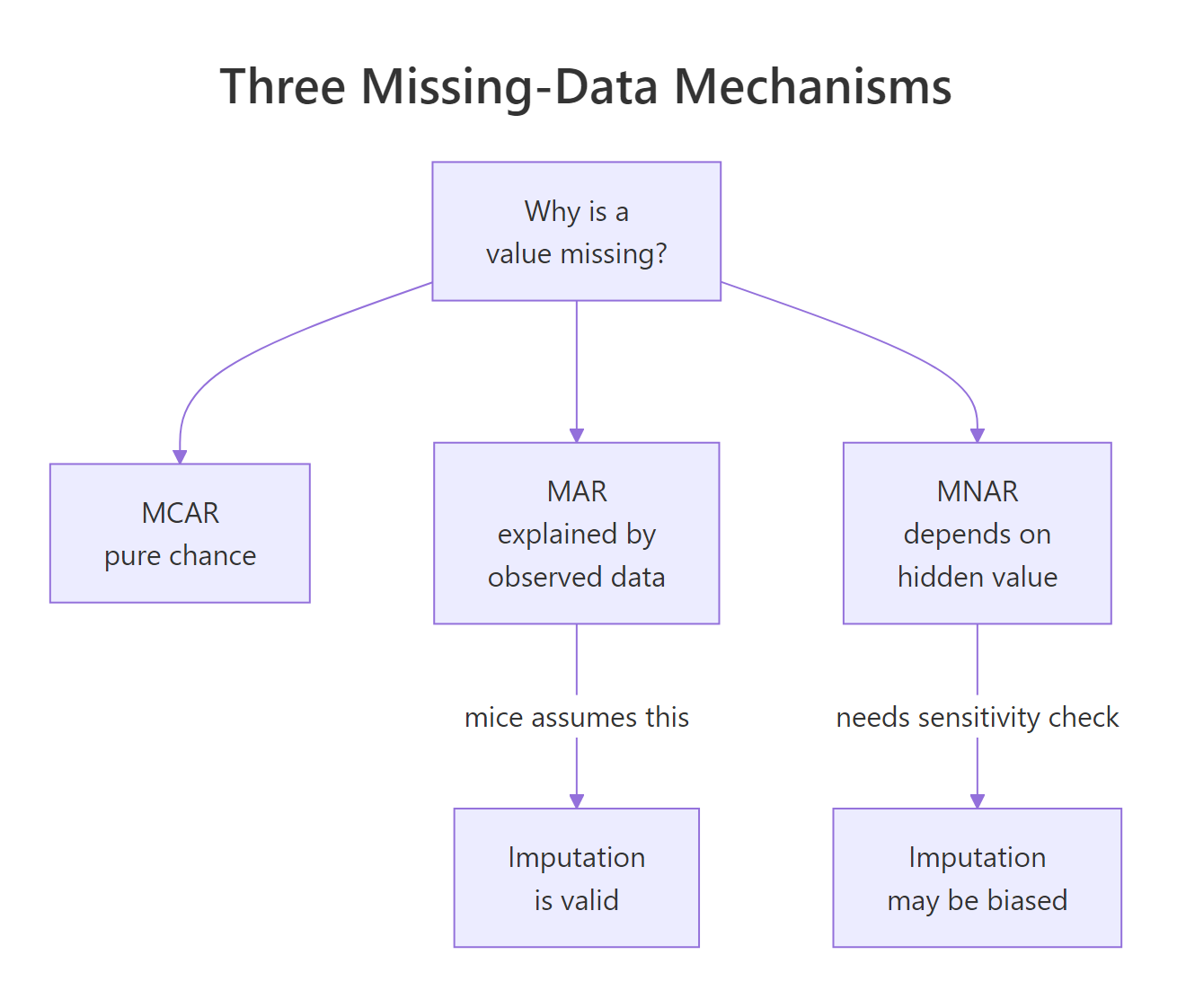
Figure 3: The three missing-data mechanisms and what each means for imputation.
The three mechanisms are easiest to grasp through a single example: a scale that sometimes fails to record a person's weight.
| Mechanism | Why the value is missing | What to do |
|---|---|---|
| MCAR | Pure chance, unrelated to anything (a random battery failure) | Deletion is unbiased; imputation adds efficiency |
| MAR | Explained by other observed columns (older scales fail more, and you recorded scale age) | Multiple imputation is valid |
| MNAR | Depends on the hidden value itself (heavier people skip weighing) | Imputation can be biased; needs a sensitivity check |
Multiple imputation assumes MAR, meaning the reason a value is missing can be explained by the columns you did observe. You can probe this a little. If the days with missing ozone differ systematically from other days on the variables you do see, then missingness is clearly not pure chance.
Here the average temperature is essentially the same (77.9) whether ozone was recorded or not, so temperature gives no hint about why ozone went missing. That is reassuring, but note the catch: this test can only inspect the variables you observed. It can never see whether missingness depended on the unrecorded ozone value itself, which is exactly the MNAR case.
Two practical habits make the MAR assumption more believable. First, feed mice every variable that might explain the missingness, including extra "auxiliary" columns you will not model later, because more context makes MAR more plausible. Second, use enough imputations. A common rule of thumb sets m at least as high as the percentage of incomplete rows, so with 27 percent incomplete here, m around 20 to 30 is safer than the 5 we used for speed.
Try it: Run the same probe for Wind instead of Temp. Do windy days differ in how often ozone is missing?
Click to reveal solution
Explanation: Days with missing ozone were slightly windier on average (10.3 versus 9.9). A mild signal like this is a reason to keep Wind in the imputation model, which mice already does by default.
Practice Exercises
These combine several steps of the workflow. Each solution runs in a local R session because it uses the mice package. Use fresh variable names so you do not overwrite the objects from the tutorial.
Exercise 1: Impute more and flip the model around
Create 10 imputations of airquality, then pool a model that predicts Temp from Ozone and Wind. Report the pooled coefficients. Use seed = 500.
# Hint: mice(airquality, m = 10, seed = 500, printFlag = FALSE)
# then with(..., lm(Temp ~ Ozone + Wind)) and pool().

# Write your code below:
Click to reveal solution
my_imp <- mice(airquality, m = 10, method = "pmm", seed = 500, printFlag = FALSE)
my_fit <- with(my_imp, lm(Temp ~ Ozone + Wind))
my_res <- summary(pool(my_fit))
data.frame(term = my_res$term,
           estimate = round(my_res$estimate, 3),
           std.error = round(my_res$std.error, 3),
           p.value = round(my_res$p.value, 4))
#>          term estimate std.error p.value
#> 1 (Intercept)   73.403     2.729  0.0000
#> 2       Ozone    0.181     0.023  0.0000
#> 3        Wind   -0.304     0.200  0.1309
Explanation: Each extra unit of ozone is linked to about 0.181 degrees more warmth, and with 10 imputations the pooled standard errors are a touch more stable than with 5.
Exercise 2: Control which predictors mice uses
By default mice uses every other column to impute each variable, including Day, which is just a calendar index. Use quickpred() to build a predictor matrix that drops weak predictors, inspect the row for Ozone, then re-impute and pool the main model.
# Hint: pred <- quickpred(airquality); look at pred["Ozone", ].
# Then mice(airquality, predictorMatrix = pred, ...).

# Write your code below:
Click to reveal solution
pred <- quickpred(airquality)
pred["Ozone", ]
#>   Ozone Solar.R    Wind    Temp   Month     Day
#>       0       1       1       1       1       0

imp_cust <- mice(airquality, predictorMatrix = pred, m = 5, seed = 99, printFlag = FALSE)
cust_res <- summary(pool(with(imp_cust, lm(Ozone ~ Temp + Wind + Solar.R))))
data.frame(term = cust_res$term,
           estimate = round(cust_res$estimate, 3),
           std.error = round(cust_res$std.error, 3))
#>          term estimate std.error
#> 1 (Intercept)  -65.827    21.692
#> 2        Temp    1.622     0.235
#> 3        Wind   -2.946     0.640
#> 4     Solar.R    0.058     0.022
Explanation: quickpred() dropped Day (a 0 in the row) because it barely correlates with ozone. The pooled estimates barely move, which is reassuring: the imputation was not leaning on a useless predictor.
Exercise 3: Put a number on what deletion cost you
Compare the Temp standard error from the complete-case model (cc_model, fit at the top of this guide) against the pooled multiple-imputation standard error (pooled). Which is smaller, and why?
# Hint: pull "Std. Error" for Temp from summary(cc_model)$coefficients,
# and std.error for Temp from summary(pooled).

# Write your code below:
Click to reveal solution
cc_se <- round(summary(cc_model)$coefficients["Temp", "Std. Error"], 3)
mi_se <- round(summary(pooled)$std.error[summary(pooled)$term == "Temp"], 3)
c(complete_case_SE = cc_se, multiple_imputation_SE = mi_se)
#>       complete_case_SE multiple_imputation_SE
#>                  0.254                  0.241
Explanation: The multiple-imputation standard error (0.241) is smaller than the complete-case one (0.254). By keeping all 153 rows instead of dropping 42, imputation recovered information that deletion threw away, while still accounting for the uncertainty of the fills.
Frequently Asked Questions
How many imputations should I use?
Five is fine for a first pass, but for a result you will report, use more. A widely used rule of thumb sets m at least as high as the percentage of rows with any missing value. More imputations reduce simulation noise and stabilize the standard errors, with diminishing returns past roughly 20 to 50.
Should I impute the outcome variable?
Yes. It is valid to let mice impute the outcome along with everything else, and dropping outcome-missing rows beforehand can bias your results. The one exception is when a row is missing the outcome and offers no other useful information, in which case it contributes little either way.
What is pmm, and when should I change it?
Predictive mean matching (pmm) borrows a real observed value from a similar row, so it is a safe default for numeric columns and keeps imputations plausible. Switch methods by variable type: use logreg for a binary factor, polyreg for an unordered categorical, and polr for an ordered categorical.
How does mice handle categorical variables?
Store them as R factors before imputing, and mice picks a suitable method automatically. A two-level factor gets logistic regression, an unordered factor gets multinomial regression, and an ordered factor gets proportional-odds regression.
Do I need to check convergence every time?
It is a cheap habit worth keeping. Glance at plot(imp) for drift or separating chains, and if you see either, raise maxit to give the algorithm more cycles. For most tidy datasets the default handful of iterations is plenty.
Can mice impute interactions or squared terms?
Impute the raw variables first, then build interactions and polynomials from the completed data, or use passive imputation to keep a derived column consistent with its inputs. Imputing a product term directly usually distorts the relationship you care about.
Summary
Multiple imputation replaces each missing value with several plausible values, analyzes every version, and pools the answers so your uncertainty stays honest. The table below contrasts it with the shortcuts it replaces.
| Approach | Effect on the estimate | Effect on the standard error |
|---|---|---|
| Listwise deletion | Unbiased under MCAR, but wastes data | Inflated by the smaller sample |
| Single mean imputation | Biased toward zero | Falsely small (overconfident) |
| Multiple imputation | Recovers the honest estimate | Reflects true uncertainty |
The mice workflow is a short, repeatable loop: inspect the pattern with md.pattern(), impute with mice(), analyze each dataset with with(), combine with pool(), then check convergence and plausibility. The diagram below shows the whole path at a glance.
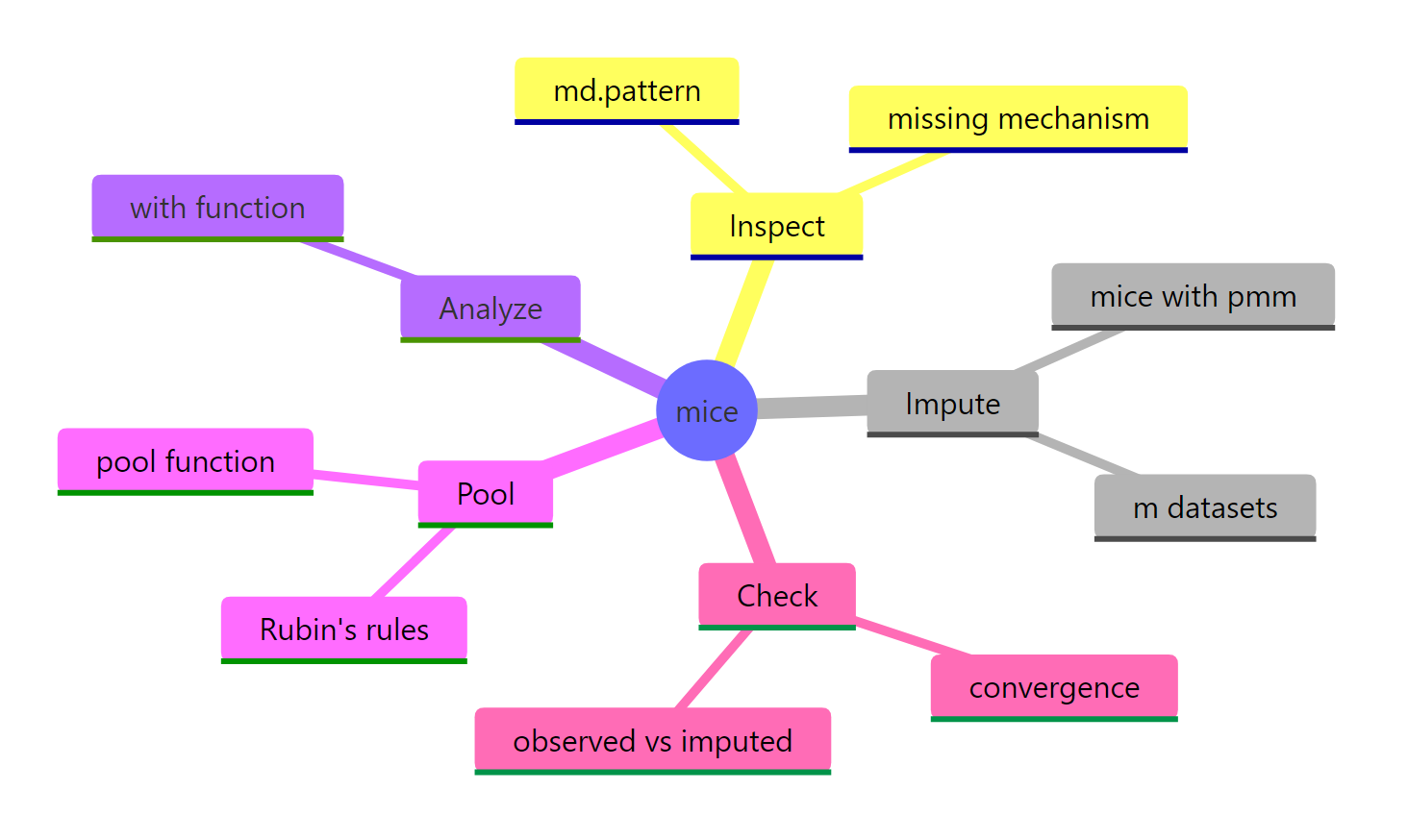
Figure 4: The mice workflow at a glance, from inspecting the missingness to checking the imputations.
Keep three things in mind. Impute enough times (let m grow with the amount of missingness), feed the imputation model every variable that might explain the gaps, and remember that the whole method rests on the MAR assumption you can reason about but never fully test.
References
- van Buuren, S. Flexible Imputation of Missing Data, 2nd Edition. CRC Press (2018). The definitive open-access book on mice. Link
- van Buuren, S. & Groothuis-Oudshoorn, K. mice: Multivariate Imputation by Chained Equations in R. Journal of Statistical Software, 45(3) (2011). Link
- mice package on CRAN. Reference manual and vignettes. Link
- mice project documentation site (amices.org). Link
- UVA Library. Getting Started with Multiple Imputation in R. Link
- mice reference: pool(). Pooling with Rubin's rules, the procedure introduced in Rubin (1987). Link
- CRAN Task View: Missing Data. A curated map of R packages for missing-data analysis. Link
Continue Learning
- Missing Value Treatment in R: a tour of the single-imputation methods that multiple imputation improves on, useful for comparison.
- Checking Model Assumptions in R: the workflow for trusting a fitted model, a natural next step after you have imputed your data.
- Linear Regression in R: the
lm()fundamentals that the analysis step of this guide builds on.