What Statistics Is For: Questions, Evidence, Decisions

Statistics is the science of turning data into answers you can act on. It gives you a disciplined way to ask a clear question, gather evidence, and then decide what to do, even when the data is noisy and incomplete.

By Selva Prabhakaran · July 2026

Code examples run against R 4.6.0

Every chart, poll, medical trial, and pricing test you have ever seen is doing the same three things underneath. It starts with a question, gathers evidence to weigh it, then reaches a decision you can defend. This first lesson of the handbook shows you that whole arc with tiny, runnable examples so the rest of your statistics journey feels like filling in details rather than learning a new language. You will write real R here, but no prior statistics is assumed. We use plain base R throughout, so nothing extra needs installing.

What problem does statistics actually solve?

The hardest questions we ask are about things we cannot fully see. A shop owner cannot watch every customer. A doctor cannot test a drug on every patient. So we collect a slice of data as evidence and reason carefully from that slice to the bigger picture. Statistics is the set of tools that makes this reasoning honest instead of wishful.

Let's make that concrete right away. Suppose you run a small online store and want to answer one question: what does a typical order look like? Here are 15 order values from last week, in dollars. We will store them in a vector and ask R for the average.

RSummarize last week's orders

orders <- c(23, 41, 18, 52, 29, 37, 44, 25, 33, 60, 21, 39, 48, 27, 35) mean(orders) #> [1] 35.46667

That single number, about 35.47 dollars, is your first piece of statistics. The mean() function added up all 15 values and divided by 15. Instead of squinting at a list of numbers, you now have one summary that answers "what is typical here?" in a way you can put in a report or use to plan.

That is the whole game in miniature. You had a question (what is a typical order?), you had evidence (the 15 values), and you produced an answer you can act on. Every technique in this handbook is a more careful version of that same loop.

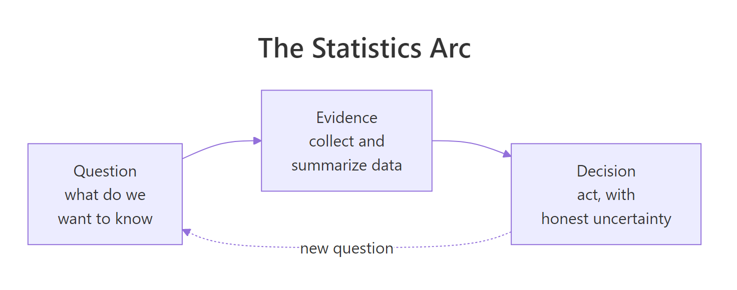
Diagram showing the loop from a question to evidence to a decision and back to a new question

Figure 1: Statistics is the loop from a question, through evidence, to a decision.

Key Insight

A single number is only an answer once you know how much to trust it. The average order was 35.47 dollars last week, but next week's 15 orders will give a different average. Most of statistics exists to measure that wiggle so you know whether a number is solid or shaky.

Try it: The average can be pulled around by one unusually large or small order. A sturdier "typical value" is the median, the middle value once the numbers are sorted. Compute the median of orders.

RYour turn: find the middle order value

# 'orders' is already available from the block above. # The median is the middle value when the numbers are sorted. # Write one line that returns it, then run the block. # your code here

Click to reveal solution

RMedian of the orders

median(orders) #> [1] 35

Explanation: median() sorts the 15 values and returns the middle one. Here it is 35, very close to the mean of 35.47, which tells you the orders are fairly balanced with no wild outlier tugging the average.

How do you turn a real-world question into one data can answer?

A question like "are my customers spending more?" is too fuzzy for data to answer directly. Statistics starts by sharpening it into three plain pieces: the thing you measure, the group you care about, plus one number that summarizes them.

The thing you measure is the variable, here the dollar value of an order. The group you care about is the population, here every order your store will ever get, which you can never fully see. The handful you actually measure is the sample. A number computed from the whole population (its true average) is called a parameter, and the matching number computed from your sample is a statistic. The sample statistic is your best estimate of the population parameter.

Let's watch that estimate in action. We will pretend, just for teaching, that we can see the whole population of 2000 past orders. In real life you never can, which is exactly why sampling matters. We then take a small sample of 15 and compare the sample's average to the population's average.

RDraw a sample from a population

set.seed(1) population <- round(rnorm(2000, mean = 35, sd = 12)) sample_orders <- sample(population, size = 15) c(population_mean = mean(population), sample_mean = mean(sample_orders)) #> population_mean sample_mean #> 34.83250 36.66667

Read the output as two labelled numbers. The population_mean of 34.83 is the truth we are chasing. The sample_mean of 36.67 is our estimate from just 15 orders. They are close but not identical, and that small gap is the heart of the whole subject. Your sample gives you a good guess, not the exact answer.

The set.seed(1) line makes the random draw repeatable, so you get the same numbers every time you run it. rnorm() invented 2000 realistic order values, and sample() picked 15 of them at random.

Diagram showing a population narrowing to a sample and then to a computed statistic that estimates the true parameter

Figure 2: A statistic from a sample is our best estimate of a population parameter.

Note

We almost never measure the whole population. In practice you only ever hold a sample, so every headline number you compute is an estimate. Keeping the population-versus-sample distinction in mind is what stops you from over-trusting a single figure.

Try it: A different random sample would give a different estimate. Draw a fresh sample of 15 from population using set.seed(99) and report its mean.

RYour turn: take a second sample

# Reuse 'population' from the block above. # Set a new seed, draw 15 values with sample(), then take the mean. # your code here

Click to reveal solution

RA second sample gives a different estimate

set.seed(99) another_sample <- sample(population, size = 15) mean(another_sample) #> [1] 32.06667

Explanation: This sample averages 32.07, versus 36.67 from the first sample, even though both come from the same population. Same truth, different samples, different estimates. That spread is the reason we need the tools in the rest of this lesson.

What is the difference between descriptive and inferential statistics?

Now that you have seen a sample estimate a population, the two big branches of statistics fall into place naturally. Descriptive statistics summarize the data you actually have. Inferential statistics use that sample to make a careful claim about the wider population you cannot see.

Here is the same idea as a table you can keep as a mental map.

Question it answers	Branch	What you do	Example from this post
What happened in the data I have?	Descriptive	Summarize with a center and a spread	The 15 orders averaged 35.47
What is likely true beyond my data?	Inferential	Estimate a population value with a margin	All customers average about 36.67, give or take 5.78

Let's do both jobs on the same sample. The descriptive part is just the sample mean. The inferential part attaches a "give or take" to that mean, a range that reflects how much a sample of this size could wobble. The wobble is measured by the standard error, which is the spread of the data divided by the square root of the sample size.

RDescribe the sample, then infer about everyone

mean(sample_orders) se <- sd(sample_orders) / sqrt(length(sample_orders)) c(estimate = mean(sample_orders), give_or_take = 1.96 * se) #> [1] 36.66667 #> estimate give_or_take #> 36.666667 5.781697

The first line is descriptive: the sample averaged 36.67. The second calculation is inferential: our best estimate for all customers is 36.67, give or take about 5.78 dollars. So the plausible range runs roughly from 31 to 42 dollars. The 1.96 is a conventional multiplier for a 95 percent range: stretch the standard error by 1.96 on each side and you cover where the true average sits about 95 percent of the time. You will see exactly where that number comes from later, so for now just read it as "the width of a 95 percent margin". That give-or-take is honesty made numeric. It admits that 15 orders cannot pin down the true average exactly.

This give-or-take is a gentle preview of the confidence interval, which you will meet properly later. For now, just hold the idea: an inferential answer is an estimate plus a range, never a bare number pretending to be exact.

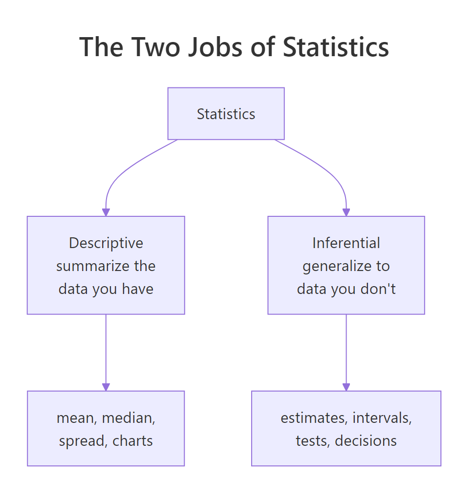
Diagram splitting statistics into a descriptive branch that summarizes data and an inferential branch that generalizes to a population

Figure 3: Descriptive statistics summarize your data; inferential statistics generalize beyond it.

Try it: Put a give-or-take on last week's real orders. Compute the standard error, then report the mean and 1.96 times the standard error together.

RYour turn: add a margin to the orders average

# Reuse 'orders'. Standard error = sd(orders) / sqrt(number of orders). # Then combine mean(orders) and 1.96 * se into one c(...). # your code here

Click to reveal solution

REstimate and margin for the orders

se_orders <- sd(orders) / sqrt(length(orders)) c(estimate = mean(orders), give_or_take = 1.96 * se_orders) #> estimate give_or_take #> 35.466667 6.123435

Explanation: Last week's typical order was 35.47 dollars, give or take about 6.12. With only 15 orders the margin is wide, which is the data telling you honestly that it cannot promise more precision yet.

How do you summarize evidence with descriptive statistics?

Good descriptive statistics answer two questions about any batch of numbers: where is the center, and how spread out are they? A center without a spread is half a picture. Two stores can both average 35 dollars per order while one is steady and the other swings wildly.

Let's measure both at once. We will report the mean and median for the center, and the standard deviation and range for the spread. The standard deviation is the typical distance of a value from the mean, and the range is simply the largest value minus the smallest.

RMeasure center and spread together

c(mean = mean(orders), median = median(orders), sd = sd(orders), range = diff(range(orders))) #> mean median sd range #> 35.46667 35.00000 12.09998 42.00000

Now you have a fuller portrait. The center sits around 35 dollars, orders typically land about 12 dollars away from that center, and the gap between the cheapest and priciest order is 42 dollars. That spread is as important as the average when you plan inventory or set expectations.

Center and spread also warn you when the mean is misleading. Watch what one unusual order does. We will add a single 900 dollar corporate order to the batch and recompute the mean and median.

RHow one outlier pulls the mean

orders_vip <- c(orders, 900) c(mean = mean(orders_vip), median = median(orders_vip)) #> mean median #> 89.5 36.0

One order rewrote the story. The mean leapt from 35.47 to 89.5 dollars, a "typical" order that no actual customer placed. The median barely moved, from 35 to 36. The median stayed put because it depends only on the value in the middle position, not on how large the extreme value is.

Warning

The mean is easily dragged by outliers, the median is not. For skewed data such as incomes, house prices, or order values with a few whales, report the median as your typical value and treat a lone mean with suspicion.

Try it: Given exam scores where one value is a typo, decide which summary is more representative. Compute the mean and median of c(70, 72, 68, 75, 71, 69, 300).

RYour turn: spot the misleading average

# Store the scores in a vector, then compute mean and median together. # One score is clearly a data-entry error. Which summary survives it? # your code here

Click to reveal solution

RMean versus median with a typo

ex_scores <- c(70, 72, 68, 75, 71, 69, 300) c(mean = mean(ex_scores), median = median(ex_scores)) #> mean median #> 103.5714 71.0000

Explanation: The bogus 300 drags the mean up to 103.57, higher than every real score. The median stays at 71, right in the pack. When you suspect bad or extreme values, trust the median.

Why can a sample fool you?

Here is the single most important idea in the whole subject. Any one sample is just one lucky or unlucky draw, so the number you compute from it wobbles from sample to sample. Statistics exists to measure that wobble, because until you know how big it is, you cannot tell a real signal from random noise.

Let's see the wobble directly. We will take ten fresh samples of 15 orders each from the same population and record each sample's mean. If samples told the whole truth, all ten means would be identical.

RWatch the sample mean wobble

set.seed(42) sample_means <- replicate(10, mean(sample(population, 15))) round(sample_means, 1) #> [1] 36.0 30.1 33.7 40.2 30.8 35.5 32.1 34.7 36.5 36.4

The true population average is 34.83, yet these ten estimates range from 30.1 all the way to 40.2. Nobody made a mistake. This is just what happens when you peek at 15 orders at a time. A single sample could easily have handed you 30.1 or 40.2 and looked perfectly convincing.

So can you tame the wobble? Yes, by collecting more data. Let's compare the spread of sample means when each sample has 15 orders versus 200 orders. We measure "spread of the estimates" with the standard deviation of the many sample means.

RBigger samples wobble less

set.seed(42) small <- replicate(1000, mean(sample(population, 15))) large <- replicate(1000, mean(sample(population, 200))) c(spread_n15 = sd(small), spread_n200 = sd(large)) #> spread_n15 spread_n200 #> 3.0963779 0.8088035

With 15 orders per sample the estimates scatter by about 3.1 dollars. Bump each sample to 200 orders and the scatter shrinks to about 0.81. More evidence means a steadier estimate. The collection of all these sample means even has a name, the sampling distribution, and it is the bridge to nearly every inference technique.

Key Insight

Statistics measures how much a number would wobble, so you know how much to trust it. A mean of 36 from 15 orders and a mean of 36 from 2000 orders are not equally believable, and the amount of wobble is exactly what tells them apart.

Try it: If bigger samples wobble less, tiny samples should wobble more. Repeat the wobble measurement with samples of only 5 orders and compare it to the 3.1 you saw for 15.

RYour turn: shrink the sample to 5

# Reuse 'population'. Take 1000 sample means, each from a sample of size 5, # then report their standard deviation. # your code here

Click to reveal solution

RWobble with samples of size 5

set.seed(42) tiny <- replicate(1000, mean(sample(population, 5))) sd(tiny) #> [1] 5.643031

Explanation: With only 5 orders per sample the estimates scatter by about 5.64, much more than the 3.1 for samples of 15. Small samples are jumpy, which is why a claim built on a handful of observations deserves extra caution.

How does statistics turn evidence into a decision?

Most real questions compare two things. Did the new checkout page make people spend more than the old one? You will always see some difference between two groups, because random wobble guarantees it. The job of statistics is to judge whether the difference is bigger than the noise, so you can decide with your eyes open.

Let's set up the comparison. We collect 40 orders from the old checkout and 40 from the new one, then look at the gap between their averages.

RCompare the old and new checkout

set.seed(7) old <- round(rnorm(40, mean = 35, sd = 12)) new <- round(rnorm(40, mean = 40, sd = 12)) c(old_mean = mean(old), new_mean = mean(new), difference = mean(new) - mean(old)) #> old_mean new_mean difference #> 38.250 41.425 3.175

The new checkout looks better: its orders averaged 41.43 dollars against 38.25 for the old one, a difference of 3.18. It is tempting to declare victory and ship it. But you just watched sample means swing by several dollars for no reason at all, so the honest next question is: could a gap of 3.18 be pure noise?

We can answer that with a simple, powerful trick. If the checkout truly made no difference, then the labels "old" and "new" are meaningless and we could shuffle them freely. So we pool all 80 orders, reshuffle the labels thousands of times, and see how often chance alone produces a gap as big as the 3.18 we actually saw.

RCould the gap be just noise?

set.seed(7) observed <- mean(new) - mean(old) pooled <- c(old, new) fake_gaps <- replicate(2000, { shuffled <- sample(pooled) mean(shuffled[1:40]) - mean(shuffled[41:80]) }) mean(abs(fake_gaps) >= abs(observed)) #> [1] 0.2235

Read that result carefully: about 22 percent of the time, random shuffling alone produced a gap at least as big as our 3.18. That is not rare. When pure chance can imitate your result almost a quarter of the time, you do not have strong evidence that the new checkout is better. The responsible decision is not "ship it", it is "keep collecting orders before deciding".

That proportion, the share of chance results as extreme as yours, is the seed of a hypothesis test and its famous p-value. You will formalize it later, but you have already grasped the core idea by building it yourself.

Warning

A visible difference is not automatically a real one. Two ways to be wrong sit on either side of every decision: calling a chance blip a real effect (a false alarm), or missing a genuine effect because you had too little data. Good statistics is the discipline of balancing those two mistakes instead of just eyeballing the bigger number.

Try it: The mean can be swayed by a few large orders, so recompute the comparison using medians. Report the old median, the new median, then the gap between them.

RYour turn: compare with medians instead

# Reuse 'old' and 'new'. Compute median(old), median(new), # and their difference, all inside one c(...). # your code here

Click to reveal solution

RComparing medians

c(old_median = median(old), new_median = median(new), median_gap = median(new) - median(old)) #> old_median new_median median_gap #> 37 42 5

Explanation: The median gap of 5 dollars is even larger than the mean gap of 3.18, which is worth noticing, but by itself it still does not prove the new checkout wins. The same shuffle test would be needed to judge whether a median gap this size is beyond noise.

Putting it together: an end-to-end example

Let's run the full arc once more on a completely different question, so you can see that the pattern travels. A school tries a new teaching method and asks: did exam scores actually improve? We measure 30 students under the old method and 30 under the new one, then look at the gap.

RDid the new teaching method raise scores?

set.seed(2024) method_a <- round(rnorm(30, mean = 68, sd = 10)) method_b <- round(rnorm(30, mean = 74, sd = 10)) c(mean_a = mean(method_a), mean_b = mean(method_b), gap = mean(method_b) - mean(method_a)) #> mean_a mean_b gap #> 65.933333 73.700000 7.766667

The new method scored 73.7 on average against 65.9 for the old one, a gap of 7.77 points. As before, we refuse to trust our eyes and ask whether chance could fake a gap this big. Same shuffle test, new data.

RIs the score gap beyond chance?

gap <- mean(method_b) - mean(method_a) pooled_scores <- c(method_a, method_b) set.seed(2024) chance_gaps <- replicate(2000, { s <- sample(pooled_scores) mean(s[1:30]) - mean(s[31:60]) }) mean(abs(chance_gaps) >= abs(gap)) #> [1] 0.006

This time the verdict is completely different. Random shuffling produced a gap as big as 7.77 only about 0.6 percent of the time. Chance can barely imitate this result, so you have strong evidence the new method genuinely helped, and the sensible decision is to adopt it and keep monitoring.

Notice the contrast with the checkout example. There, a gap could be reproduced by chance 22 percent of the time, so we held off. Here, chance reproduces the gap under 1 percent of the time, so we act. The number you compute is only the start; the decision comes from weighing it against the noise. That single habit, comparing the signal to the noise before you commit, is what statistical thinking really means.

Practice Exercises

These combine several ideas from the lesson. Try each one before opening the solution. The exercises use their own variable names, so they will not disturb the objects from the tutorial above.

Exercise 1: Describe a noisy metric

You track daily website visitors for ten days: 220, 240, 235, 500, 225, 230, 245, 238, 228, 233. One day had a traffic spike from a viral post. Report the mean, the median, and a give-or-take margin (1.96 times the standard error) for the average, then decide which center you would quote to your boss.

RExercise 1 starter

# Store the ten counts in my_visitors. # Compute the standard error, then report mean, median, and 1.96 * se together. # your code here

Click to reveal solution

RExercise 1 solution

my_visitors <- c(220, 240, 235, 500, 225, 230, 245, 238, 228, 233) my_se <- sd(my_visitors) / sqrt(length(my_visitors)) c(mean = mean(my_visitors), median = median(my_visitors), give_or_take = 1.96 * my_se) #> mean median give_or_take #> 259.40000 234.00000 52.59573

Explanation: The viral day drags the mean up to 259 and blows the margin out to nearly 53, because one extreme value inflates both the average and the spread. The median of 234 describes a normal day far better. Quote the median.

Exercise 2: How much does sample size tame the wobble?

Create a population of 5000 values with rnorm(5000, mean = 50, sd = 15) using set.seed(303). Estimate the wobble (the standard deviation of 1000 sample means) for samples of size 25 and size 100, then report their ratio. Roughly how many times more data do you need to cut the wobble in half?

RExercise 2 starter

# Build my_pop, then compute the sd of 1000 sample means for n = 25 and n = 100. # Finally report both wobbles and their ratio. # your code here

Click to reveal solution

RExercise 2 solution

set.seed(303) my_pop <- rnorm(5000, mean = 50, sd = 15) wobble_25 <- sd(replicate(1000, mean(sample(my_pop, 25)))) wobble_100 <- sd(replicate(1000, mean(sample(my_pop, 100)))) c(n25 = wobble_25, n100 = wobble_100, ratio = wobble_25 / wobble_100) #> n25 n100 ratio #> 2.853473 1.505573 1.895274

Explanation: Quadrupling the sample size from 25 to 100 cut the wobble roughly in half (the ratio is about 1.9, close to 2). This is the famous square-root rule: to halve your uncertainty you need about four times the data, not twice.

Exercise 3: Signal or noise?

A team compares a control group and a treatment group, each with 50 people. Generate them with set.seed(88): control is round(rnorm(50, mean = 100, sd = 20)) and treatment is round(rnorm(50, mean = 108, sd = 20)). Measure the observed gap in means, then run a shuffle test with 3000 reshuffles to find the share of chance gaps at least as big as the observed one. Would you call the effect real?

RExercise 3 starter

# Build control and treatment, compute my_gap, pool them, # then reshuffle 3000 times and compute the share as big as my_gap. # your code here

Click to reveal solution

RExercise 3 solution

set.seed(88) control <- round(rnorm(50, mean = 100, sd = 20)) treatment <- round(rnorm(50, mean = 108, sd = 20)) my_gap <- mean(treatment) - mean(control) my_pool <- c(control, treatment) noise_gaps <- replicate(3000, { s <- sample(my_pool) mean(s[1:50]) - mean(s[51:100]) }) c(observed_gap = my_gap, share_as_big = mean(abs(noise_gaps) >= abs(my_gap))) #> observed_gap share_as_big #> 10.08000000 0.01266667

Explanation: The observed gap is about 10, and chance reproduces a gap that big only about 1.3 percent of the time. That is strong evidence of a real effect, so you would act on it, while still remembering that "strong evidence" is not the same as "certainty".

Summary

Statistics is not a pile of formulas. It is one repeatable habit: turn a question into something measurable, summarize the evidence, judge how much that evidence could wobble, and only then decide. Everything else in this handbook is a sharper tool for one of those four steps.

The job	The question it answers	The tool you met here
Frame	What do we want to know, and about whom?	population, sample, variable
Describe	What does the evidence actually say?	mean, median, standard deviation, range
Judge trust	How much could this number wobble?	repeated sampling, standard error
Decide	Is the signal bigger than the noise?	comparing groups, the shuffle test

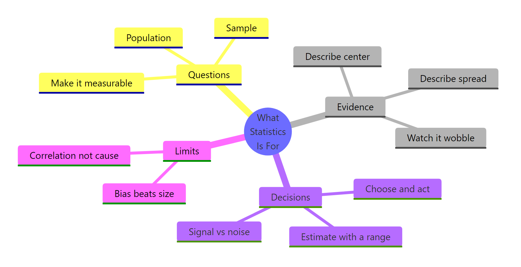
Mindmap summarizing the four ideas of the lesson: framing questions, gathering evidence, making decisions, and respecting limits

Figure 4: The whole lesson on one page: framing questions, weighing evidence, deciding under noise, respecting the limits.

Frequently Asked Questions

Is statistics just a branch of mathematics?

Mathematics is the toolbox, but statistics is really a way of reasoning under uncertainty. The equations matter less than the habit of asking how much you can trust a number before you act on it. That is why this lesson leaned on simulation and plain reasoning rather than heavy formulas.

Should I learn descriptive or inferential statistics first?

Descriptive first, always. You need to summarize a batch of numbers with a center and a spread before it makes any sense to generalize from a sample to a population. This handbook follows that order, and so should your own analyses.

How much data is enough?

There is no single magic number, because it depends on how much your measurements wobble and how small an effect you care about. The useful move is the one you practiced here: estimate the wobble by resampling, and collect more data when the wobble is large relative to the effect you are chasing.

Can statistics prove that something is true?

No, and that honesty is its strength. Statistics measures how strongly the evidence points one way, so you can act sensibly, but it never delivers certainty. A tiny share of chance-produced results as extreme as yours means "strong evidence", not "proof".

Do I need to be good at math to learn statistics?

You need comfort with basic arithmetic and a willingness to think carefully, not advanced math. Every idea in this lesson came through small code examples and everyday reasoning. As the handbook grows you will pick up notation gradually, always after you have seen the idea work in code first.

References

Diez, D., Cetinkaya-Rundel, M., and Barr, C. OpenIntro Statistics, 4th Edition. A free, beginner-friendly foundation. Link
R Core Team. An Introduction to R, official manual. Link
Wickham, H., Cetinkaya-Rundel, M., and Grolemund, G. R for Data Science, 2nd Edition. Link
Wasserstein, R. L., and Lazar, N. A. The ASA Statement on p-Values (2016). The American Statistician. Link
Reinhart, A. Statistics Done Wrong: The Woefully Complete Guide. Link
Kunin, D., and collaborators. Seeing Theory: A visual introduction to probability and statistics, Brown University. Link
R documentation for mean(). Link

Continue Learning

Sampling Distributions in R: the collection of sample means you watched wobble here, studied in full.
Confidence Intervals in R: the precise version of the give-or-take margin you attached to your estimates.
Hypothesis Testing in R: the formal home of the shuffle test and the p-value you built by hand.

Navigate

What Statistics Is For: Questions, Evidence, Decisions

What problem does statistics actually solve?

How do you turn a real-world question into one data can answer?

What is the difference between descriptive and inferential statistics?

How do you summarize evidence with descriptive statistics?

Why can a sample fool you?

How does statistics turn evidence into a decision?

Putting it together: an end-to-end example

Practice Exercises

Exercise 1: Describe a noisy metric

Exercise 2: How much does sample size tame the wobble?

Exercise 3: Signal or noise?

Summary

Frequently Asked Questions

Is statistics just a branch of mathematics?

Should I learn descriptive or inferential statistics first?

How much data is enough?

Can statistics prove that something is true?

Do I need to be good at math to learn statistics?

References

Continue Learning

Related Tutorials