Capstone: A Clinical-Style Group Comparison in R
A clinical-style comparison asks one clean question, does the treatment beat the control, and answers it with a discipline that separates what you decided before seeing the data from what the data suggested afterward. This capstone runs that whole workflow on one simulated two-arm trial whose true effect we already know, so every number on the page is checkable against the truth.
This is a capstone, so it stitches together skills you have met one at a time: power, a group test, effect sizes, and covariate adjustment. We will run a small blood-pressure program evaluation from protocol to final report, using base R plus a little dplyr and ggplot2. The same pattern fits any two-arm A/B comparison, a new checkout flow against the old one, a coaching program against a waitlist, so read "patient" as "unit" and "clinic" as "your team" whenever you like.
What are we comparing, and what did we lock in first?
A two-arm comparison has exactly two groups. One arm gets the new thing, here a 12-week program to lower blood pressure, and the other arm gets standard care. Everyone is randomly assigned to an arm, and we compare a single agreed-on number between the two. That number, and the exact way we will compare it, are decided before we see a single result. Writing those rules down first is preregistration in miniature, and it is what stops us from fishing for a story after the fact.
Let us make "decided in advance" concrete by storing the protocol as a small table and printing it. Everything below flows from these six decisions.
That table is the contract. The primary endpoint is the one outcome that decides success, systolic blood pressure (SBP) at week 12. The analysis set is intention-to-treat, meaning we analyze people in the arm they were randomized to, no matter what they actually did later. Alpha is our error budget for a false positive, set at the usual 0.05. The minimally important difference, 5 mmHg, is the smallest change we would call clinically worth having.
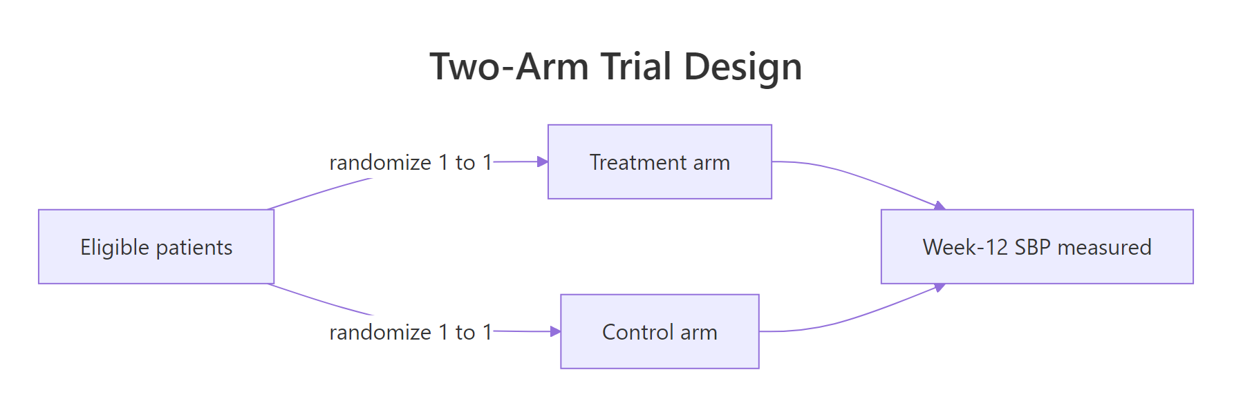
Figure 1: The two-arm parallel design: randomize once, measure the same endpoint in both arms.
Try it: A protocol needs its endpoints written down. Build a small data frame called ex_endpoints with a type column ("Primary", "Secondary", "Secondary") and an endpoint column naming the week-12 SBP as primary and two sensible secondaries.
Click to reveal solution
Explanation: Secondary endpoints support the story but never overrule the primary. Reaching a clinical target (SBP below 130) and the raw change from baseline are natural companions to the primary week-12 level.
How many patients do we need, and how did we decide?
Sample size is not a guess, it is a calculation you do before enrolling anyone. You feed in three numbers you already committed to: the smallest difference worth detecting (our 5 mmHg), how spread out the outcome is (its standard deviation), and the power you want, which is the chance of detecting a real effect if it exists. The convention is 80% power. R turns those into a required sample size with power.t.test().
R tells us we need about 142 people per arm to have an 80% chance of detecting a 5 mmHg difference when the outcome has a standard deviation of 15 mmHg. We will round up and enroll 150 per arm to leave room for dropout. Notice how the answer depends entirely on assumptions we chose in advance, not on any data.
To build intuition, let us watch power climb as the sample grows. We sweep a range of per-arm sizes and read off the power for each.
At 60 per arm we would miss a real 5 mmHg effect more than half the time. By 140 per arm we cross the 80% line, which matches the 142 the formula gave us. The same numbers are easier to feel as a curve, so let us draw it.
The dashed line is our 80% target, and the curve shows the sample size where we clear it. The curve is steep on the left and flat on the right: past a point, buying more patients barely buys more power, which is useful when a budget is tight.
Try it: Suppose you only care about detecting a larger 8 mmHg difference (same SD of 15, same 80% power). Use power.t.test() to find the required sample size per arm. Do you need more people or fewer?
Click to reveal solution
Explanation: A larger effect is easier to see, so it needs fewer people, only 57 per arm here versus 142 for a 5 mmHg effect. Bigger effects are cheaper to detect.
Are the two groups comparable at baseline?
Now the trial runs. We enroll 150 patients per arm and record their baseline traits: age, sex, body-mass index, and starting SBP. Because this is a simulation, we get to know the truth, and we build the data so the program truly lowers SBP by about 8 mmHg in people who stick with it. That known effect is our answer key.
We have 300 patients, split evenly. Because we drew both arms from the same recipe, they are random samples of one population, which is exactly what randomization guarantees in a real trial. Next we generate week-12 outcomes. Some patients do not adhere to the program, some drop out before week 12, and higher starting values tend to fall more (a real effect called regression to the mean). The set.seed() call makes the whole thing reproducible.
Seventeen patients have a missing week-12 value because they did not complete the study. Adherent treatment patients get the full 8 mmHg benefit; non-adherent ones get only a partial 3 mmHg; control patients get none. This is a realistic, messy data set, and it is the one our prespecified plan now has to face.
Before analyzing the outcome, we check whether randomization did its job of making the arms comparable. The right tool is the standardized mean difference (SMD): the gap between arm means measured in units of pooled spread. In symbols:
$$\text{SMD} = \frac{\bar{x}_\text{treatment} - \bar{x}_\text{control}}{\sqrt{(s^2_\text{treatment} + s^2_\text{control})/2}}$$
Where:
- $\bar{x}_\text{treatment}$ and $\bar{x}_\text{control}$ are the arm means of a baseline variable
- $s^2_\text{treatment}$ and $s^2_\text{control}$ are the arm variances
- the denominator is the pooled standard deviation of the two arms
A common rule of thumb is that an absolute SMD above 0.1 flags a noticeable imbalance. Let us build the Table 1 that every trial report opens with.
Read the SMD column. Sex, BMI, and the all-important baseline SBP sit far below 0.1, so those are well balanced. Age is the exception at 0.20: the treatment arm is about two years older by chance. That is a normal event in a trial of this size, a reminder that randomization balances groups on average, not perfectly in every single draw. The right response is not alarm and not a significance test, it is to lean on the covariate adjustment we planned for.
Try it: Compute the standardized mean difference for bmi on its own using the smd() helper defined above. Is it below the 0.1 threshold?
Click to reveal solution
Explanation: An SMD of 0.011 is essentially zero, so BMI is beautifully balanced between the arms. No test, no worry, just a number you report.
Did the treatment work? The prespecified primary analysis
This is the moment the protocol was written for. Our plan named a Welch two-sample t-test on week-12 SBP, analyzed by intention-to-treat. Intention-to-treat means we compare arms as randomized, including patients who did not fully adhere. It answers the honest, policy-relevant question, "what happens when we offer this program," rather than the flattering question, "what happens in the perfect patient." We use the observed week-12 values (a complete-case ITT), and we will account for the missing ones in the reporting section.
R compares Control against Treatment, so its confidence interval is for "Control minus Treatment" and comes out positive. That is a little awkward to read, so let us flip it to the more natural "Treatment minus Control" (a negative number means the program lowered SBP) and print a clean summary.
The program lowered week-12 SBP by 7.2 mmHg on average, with a 95% confidence interval from 4.0 to 10.4 mmHg lower. Because we built the data with a true effect near 8 mmHg (diluted a little by non-adherence), this estimate lands right where the truth is, which is reassuring. The whole interval sits below zero and beyond our 5 mmHg importance threshold at its far end, and the p-value is tiny, so by our own prespecified rule this is a clear, clinically meaningful win. The confidence interval matters more than the p-value: it tells you the plausible range of the real effect, not just that it differs from zero. If you want a refresher, see the guide on confidence intervals.
Try it: One of our secondary endpoints was the proportion of patients reaching a controlled SBP below 130 mmHg. Compute that proportion for each arm using tapply().
Click to reveal solution
Explanation: About 22% of treatment patients reached control versus 11% of controls, roughly double. Averaging a TRUE/FALSE vector gives a proportion, because R treats TRUE as 1 and FALSE as 0.
Would a different analysis change the answer?
A single test is never the whole story. A robust result should survive being poked at, so we run three sensitivity analyses and line them up against the primary. Each pokes a different assumption. This is where the "decided in advance versus data-driven" spine matters most: these were all named in the protocol as supportive analyses, so they strengthen the primary rather than replace it.
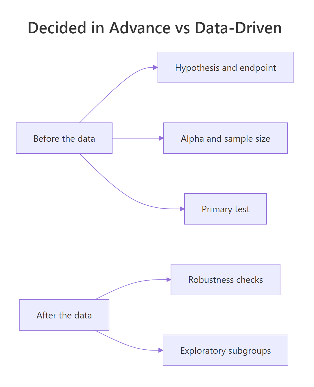
Figure 2: The spine of the chapter: what is decided before the data versus what the data drives.
The first check drops the normality assumption. The Wilcoxon rank-sum test compares the arms using ranks, not raw values, and returns a Hodges-Lehmann estimate of the typical shift between them. For more on this test, see the Mann-Whitney U test guide.
The nonparametric shift is 7.0 mmHg lower, almost identical to the primary. The second check is the most useful one in practice: ANCOVA, which is a linear model for week-12 SBP with the arm and the baseline SBP as predictors. Adjusting for the starting value soaks up a big chunk of patient-to-patient variation, which usually shrinks the confidence interval.
The armTreatment row is our adjusted effect: 7.0 mmHg lower, with a 95% interval from 8.9 to 5.0. Look at the standard error, 0.998, versus the primary test's, which we will confirm is much larger in a moment. Adjusting for baseline SBP made the estimate more precise without changing its size. The third check is per-protocol: analyze only patients who completed and adhered. This answers "how well does the program work when actually followed," a fair question, but a fragile one, because adherers are self-selected and no longer a randomized comparison.
Per-protocol shows a slightly larger 7.7 mmHg because it keeps only the full-benefit adherers. That larger number is not "more correct," it answers a different, easier question than intention-to-treat. Now line all four analyses up in one table.
Every method points the same way, an effect near 7 mmHg lower, all significant. The four estimates read even more clearly as a forest plot, where each dot is an estimate and each line is its confidence interval.
All four intervals sit entirely to the left of the dashed zero line, so no reasonable analyst would look at this and conclude "no effect." That agreement is the real prize of a sensitivity analysis.
Try it: The payoff of ANCOVA is precision. Pull the standard error of the treatment effect from the ANCOVA model and from the primary t-test, and compare them.
Click to reveal solution
Explanation: The ANCOVA standard error (0.998) is much smaller than the unadjusted one (1.629). A smaller standard error means a narrower confidence interval and more power, which is exactly why prespecified baseline adjustment is standard practice in trials.
How do we report this honestly, and what can it not claim?
A good report gives the effect in plain language, quantifies the uncertainty, and states clearly what the study cannot say. Start with a standardized effect size so readers can compare this result to studies with different scales. Cohen's d divides the raw effect by the pooled standard deviation:
$$d = \frac{\bar{x}_\text{treatment} - \bar{x}_\text{control}}{s_\text{pooled}}$$
Where $s_\text{pooled}$ is the standard deviation pooled across both arms. We convert our 7.2 mmHg effect and its interval into d.
A Cohen's d of 0.53 is a medium-sized effect by the usual convention. In plain words: "The program lowered week-12 systolic blood pressure by 7.2 mmHg on average (95% CI 4.0 to 10.4 mmHg), a medium effect of about half a standard deviation." The confidence interval carries the uncertainty, so we never report the point estimate alone. For more on choosing and reading these, see effect size in R.
Every trial report also shows where participants went, from randomization to analysis. This is the CONSORT-style flow, and reviewers expect it. We count patients at each stage from our own data.
The table tells an honest story about attrition. Both arms started at 150. Completion was similar, but the per-protocol set drops much further in the treatment arm (121 versus 138), because adherence was harder there. That gap is exactly why the per-protocol analysis is a sensitivity check and not the headline.
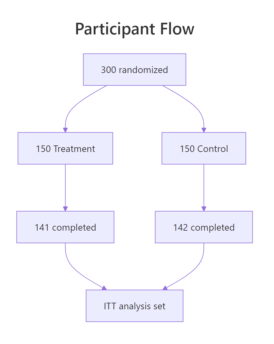
Figure 3: CONSORT-style participant flow with the real completion counts.
What can this study not claim? It cannot promise the same 7 mmHg in a different population, since our patients were sampled from one recipe. It cannot attribute the effect to any single ingredient of the program, only to the whole package versus standard care. And being one simulated trial, it stands as one piece of evidence, not a final verdict. Naming these limits is not weakness, it is what makes the positive result credible.
Try it: For the CONSORT flow you often report how many were lost to follow-up in each arm. Count the patients per arm who did not complete week 12.
Click to reveal solution
Explanation: Eight controls and nine treatment patients were lost, close to balanced, which is what you hope for. Very lopsided dropout would itself threaten the comparison.
Practice Exercises
These bring several pieces of the workflow together. Use fresh variable names so you do not overwrite the objects built above.
Exercise 1: Analyze the change from baseline
The change from baseline (week-12 SBP minus baseline SBP) is a common secondary endpoint. Using the itt data, compute the mean change for each arm and the difference between arms. Does the between-arm difference roughly match the primary effect of about 7 mmHg?
Click to reveal solution
Explanation: Control SBP fell 2.8 mmHg on its own (regression to the mean plus being in a trial), treatment fell 9.7 mmHg, and the 6.9 mmHg gap matches the primary analysis. Analyzing change and analyzing the week-12 level agree because randomization balanced the baseline.
Exercise 2: A richer ANCOVA
Our age variable showed a small chance imbalance. Fit an ANCOVA that adjusts for baseline SBP plus age and BMI, and read off the treatment estimate and its standard error. Does adding those covariates change the effect much?
Click to reveal solution
Explanation: The adjusted effect is 7.2 mmHg lower with a standard error near 1.01, essentially unchanged from the baseline-only ANCOVA. When the extra covariates are balanced, adjusting for them barely moves the estimate, which is a good sign of a stable result.
Exercise 3: Confirm your power by simulation
Trust the power calculation by testing it. Simulate 500 two-arm trials with 150 patients per arm, a true 8 mmHg effect, and an SD of 20, run a t-test on each, and report the fraction that reach significance. That fraction is the empirical power.
Click to reveal solution
Explanation: About 93% of the simulated trials detected the effect, so the design is well powered for an 8 mmHg difference at this sample size. Simulation is a general way to check power for any design, even ones with no tidy formula.
Frequently Asked Questions
What is the difference between intention-to-treat and per-protocol?
Intention-to-treat analyzes every patient in the arm they were randomized to, regardless of whether they adhered, so it preserves randomization and answers "does offering this program help." Per-protocol keeps only patients who followed the protocol, which answers "does the program help when followed" but breaks the randomized comparison because adherers self-select. Intention-to-treat is the primary analysis; per-protocol is a supporting sensitivity check.
Why should I not run a t-test on baseline characteristics?
Because both arms were randomly drawn from the same population, any baseline difference is due to chance by construction, so a significance test answers a question with no meaning. This is the Table 1 fallacy. Report standardized mean differences instead, and flag any variable with an absolute SMD above 0.1 as one you may want to adjust for.
When should I use ANCOVA instead of a plain t-test?
Use ANCOVA whenever you have a baseline measurement of the outcome (or another strong prognostic covariate) recorded before randomization. Adjusting for it removes a large share of patient-to-patient variation, which shrinks the standard error and raises power, usually without changing the point estimate. Name the covariates in the protocol so the adjustment is prespecified, not fished for.
Should the primary test be one-sided or two-sided?
Almost always two-sided. A two-sided test allows for the possibility that the treatment could help or harm, which is the honest default, and it is what regulators and journals expect. We prespecified two-sided at alpha 0.05, and you should have a strong, written reason before choosing one-sided.
Why report a confidence interval when the p-value is already tiny?
The p-value only tells you the result is unlikely under "no effect." The confidence interval tells you the range of effect sizes the data support, so you can judge whether the effect is large enough to matter, not just whether it is nonzero. A result can be highly significant yet too small to be worth acting on, and only the interval reveals that.
Does this analysis prove the program causes lower blood pressure?
Within this one randomized trial, the comparison supports a causal reading, because randomization makes the arms exchangeable at baseline. But it cannot promise the same effect in a different population, cannot credit any single component of the program, and is one study rather than a body of evidence. State those limits alongside the result.
Summary
This capstone ran a two-arm comparison the way a trial statistician would, holding a hard line between what was decided in advance and what the data suggested afterward.
| Stage | What we did | Key output |
|---|---|---|
| Protocol | Fixed hypothesis, endpoint, alpha, and primary test before data | The locked protocol table |
| Power | Sized the study from a 5 mmHg minimally important difference | 142 per arm for 80% power |
| Baseline | Compared arms with standardized mean differences, not tests | SMDs mostly below 0.1 |
| Primary | Prespecified Welch t-test, intention-to-treat | 7.2 mmHg lower (95% CI 4.0 to 10.4) |
| Robustness | Wilcoxon, ANCOVA, and per-protocol sensitivity checks | All agree near 7 mmHg |
| Reporting | Cohen's d, CONSORT flow, and honest limits | d = 0.53, medium effect |
The single most transferable idea is the spine: prespecify the endpoint, the test, and the alpha, then let the primary analysis lead and treat everything data-driven as support or exploration. That discipline is what separates a credible group comparison from a story fitted to the numbers, and it applies to any two-arm evaluation you run.
References
- R Core Team.
power.t.testdocumentation, the stats package. Link - Robinson, D., Hayes, A., and Couch, S. broom: tidy statistical model output. Link
- Pijls, B. G. The Table 1 Fallacy: significance testing of baseline covariate imbalance in randomised trials. PMC. Link
- Kassambara, A. ANCOVA in R: The Ultimate Practical Guide. Datanovia. Link
- CONSORT Group. The CONSORT Statement for reporting randomised trials. Link
- EQUATOR Network. CONSORT reporting guidelines. Link
- Wickham, H., Cetinkaya-Rundel, M., and Grolemund, G. R for Data Science, 2nd Edition. Link
Continue Learning
- Statistical Power Analysis in R goes deeper on sizing a study before you collect a single data point.
- ANCOVA in R unpacks the baseline-adjusted model that tightened our confidence interval.
- Effect Size in R explains how to choose, compute, and interpret standardized effects like Cohen's d.