Margin of Error and Sample Size Planning in R
The margin of error is the plus-or-minus attached to an estimate: it tells you how far your sample result could sit from the truth it is trying to measure. This guide builds that number from scratch in R, then flips it around to answer the question every survey starts with: how big a sample do I actually need?
We will use base R for almost everything, with one ggplot2 chart along the way. You will meet the margin of error for two of the most common estimates, a percentage and an average, plan the sample size each one needs, and then prove the whole thing works by running a quick simulation. Every code block runs right here in your browser, so you can change a number and watch the answer move.
What is the margin of error, in plain English?
You have seen the phrase in every election season: a poll reports "52% support, with a margin of error of plus or minus 3 points." That last part is the honesty clause. The pollster only asked a sample, not the whole country, so the real number could be a little higher or lower than 52%. The margin of error puts a size on "a little." It is the reach of the estimate: how far above or below your sample result the true value could plausibly sit.
Let us compute one. Imagine we polled 1,000 people and 52% of them said they support a measure. We want the margin of error at the usual 95% confidence level. The recipe is short: take the standard error of the percentage, then stretch it out by about 1.96.
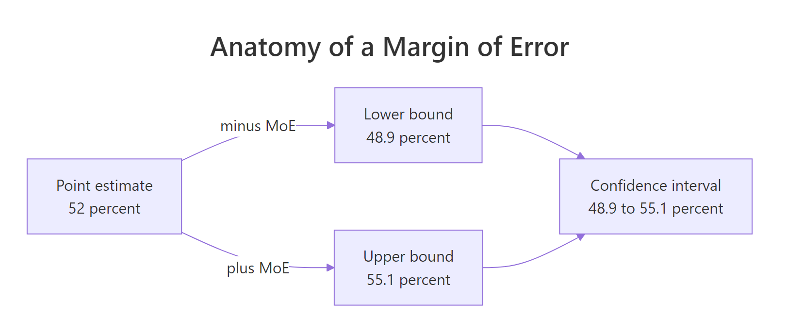
Figure 1: The margin of error is half the width of the confidence interval around the estimate.
Here is what those four numbers say. Our best guess is 52%. The margin of error came out to 0.031, or about 3.1 percentage points. Add and subtract it from the estimate and you get a lower bound of 48.9% and an upper bound of 55.1%. That pair of bounds is the confidence interval, and the margin of error is exactly half its width. So the poll is really saying: the true level of support is somewhere between roughly 49% and 55%.
Notice that the margin of error is not a mistake or a bug. It is the built-in wobble that comes from measuring a sample instead of everyone. A bigger, better-run poll would report a smaller margin of error, but no sample can shrink it to zero.
Try it: A smaller poll of 600 people found 40% support. Compute its 95% margin of error using the same recipe.
Click to reveal solution
Explanation: With 600 people the margin of error is about 3.9 points, wider than the 3.1 points from the 1,000-person poll. Fewer people means a rougher measurement and a wider plus-or-minus.
Where does the margin of error formula come from?
That number 1.96 and the square root did not fall from the sky. The margin of error is built from just two ingredients, and once you see them, every version of the formula in this guide is the same idea wearing different clothes. In words, the margin of error is a critical value multiplied by a standard error.
$$\text{MoE} = z^* \times \text{SE}$$
The standard error is how much your estimate typically bounces from sample to sample. For a percentage, it grows with how split the answers are and shrinks with how many people you ask.
$$\text{SE} = \sqrt{\frac{\hat{p}(1-\hat{p})}{n}}$$
Where:
- $z^*$ is the critical value, the multiplier that sets your confidence level
- $\text{SE}$ is the standard error, the typical bounce of the estimate
- $\hat{p}$ is your sample proportion (0.52 in the poll above)
- $n$ is the sample size
The critical value is the part you control through your confidence level. A higher confidence level means you want to be more certain the truth is inside your interval, so you reach out further, which means a bigger multiplier. R gives you the exact multiplier with qnorm(), which reads off the normal distribution. For 95% confidence you leave 2.5% in each tail, so you ask for the 97.5th percentile.
Those three numbers, 1.645, 1.96, and 2.576, are worth memorizing because you will meet them everywhere. The famous 1.96 is simply the 95% critical value. Now watch what happens to the margin of error when we keep the same poll but demand more confidence. We hold the standard error fixed and just swap in each multiplier.
Read down the last column and the trade-off is plain. If you only need 90% confidence, your margin of error is 2.6 points. Insist on 99% confidence from the same 1,000 people and the margin balloons to 4.1 points. More certainty is not free: to be surer that the truth is inside your interval, you have to make the interval wider.
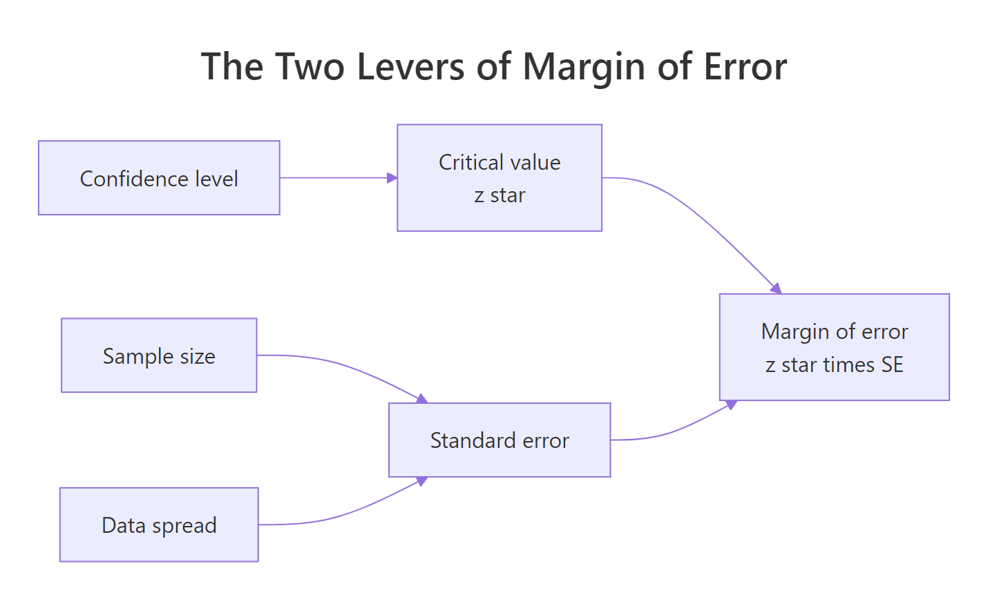
Figure 2: Two levers set the margin of error: the critical value and the standard error.
Try it: Some quick summaries use a looser 80% confidence level. Find the critical value for 80% confidence.
Click to reveal solution
Explanation: At 80% confidence the multiplier is only 1.282, smaller than the 1.96 for 95%. A lower confidence level buys you a narrower margin of error, at the cost of being right less often.
How does the margin of error behave as the sample grows?
We have pulled the confidence lever. Now let us pull the other one: sample size. Intuition says more people should mean a tighter estimate, and it does, but the payoff arrives more slowly than you might expect. To see the pattern cleanly, let us wrap the proportion margin of error in a small helper function and feed it a run of sample sizes that each quadruple the last.
Look at how the margin of error falls. At 100 people it is 9.8 points; at 400 people it is 4.9 points; at 1,600 it is 2.45 points. Each time the margin halves, the sample size has to quadruple, not double. That is the fingerprint of the square root in the formula: precision improves with the square root of your sample, so doubling your accuracy costs about four times the data.
A picture makes the shape unmistakable. Let us plot the margin of error across every sample size from 50 to 2,000.
When you run that block you get a curve that plunges steeply at first and then flattens into a long, slow tail. The early people you add help enormously; the later ones barely move the line. That flattening is exactly why polls of a few thousand people are common and polls of a hundred thousand are almost unheard of. Past a point, buying more precision is simply not worth the cost.
Try it: Use the helper to confirm the halving rule directly. Compute the margin of error at 400 and at 1,600 people and check that the second is half the first.
Click to reveal solution
Explanation: Quadrupling the sample from 400 to 1,600 cut the margin of error exactly in half, from 4.9 points to 2.45 points. Four times the people, half the wobble.
How do I plan the sample size for a target margin of error?
So far we have started with a sample size and computed the resulting margin of error. Real survey planning runs the other direction. You decide up front how precise you need to be, say "I want to be accurate to within 3 points," and you solve for the sample size that delivers it. The move is pure algebra: take the margin-of-error formula and rearrange it to put $n$ on the left.
$$n = \left(\frac{z^*}{E}\right)^2 \, p(1-p)$$
Where:
- $E$ is your target margin of error (0.03 for 3 points)
- $z^*$ is the critical value for your confidence level
- $p$ is your planning guess for the proportion
Let us turn that into a reusable function. One detail matters: a sample size must be a whole number, and rounding down would leave you just short of your target, so we always round up with ceiling().
To hit a margin of error of 3 points at 95% confidence, you need 1,068 people. That single number explains why so many national polls report roughly a thousand respondents: it is the price of a 3-point margin of error. But notice we quietly used a planning proportion of p = 0.5. Why 0.5, when we do not yet know the answer? Because 0.5 is the most pessimistic, most demanding case. The term $p(1-p)$ is largest when $p$ is one-half, so planning around 0.5 guarantees your sample is big enough no matter what the true proportion turns out to be.
The middle column peaks at 0.25 when $p$ is 0.5, and the required sample size peaks right alongside it at 1,068. A proportion near 0.1 or 0.9 is much cheaper to pin down, needing only 385 people, because lopsided splits vary less from sample to sample. When you have no prior idea what the proportion will be, plan for 0.5 and you can never be caught short.
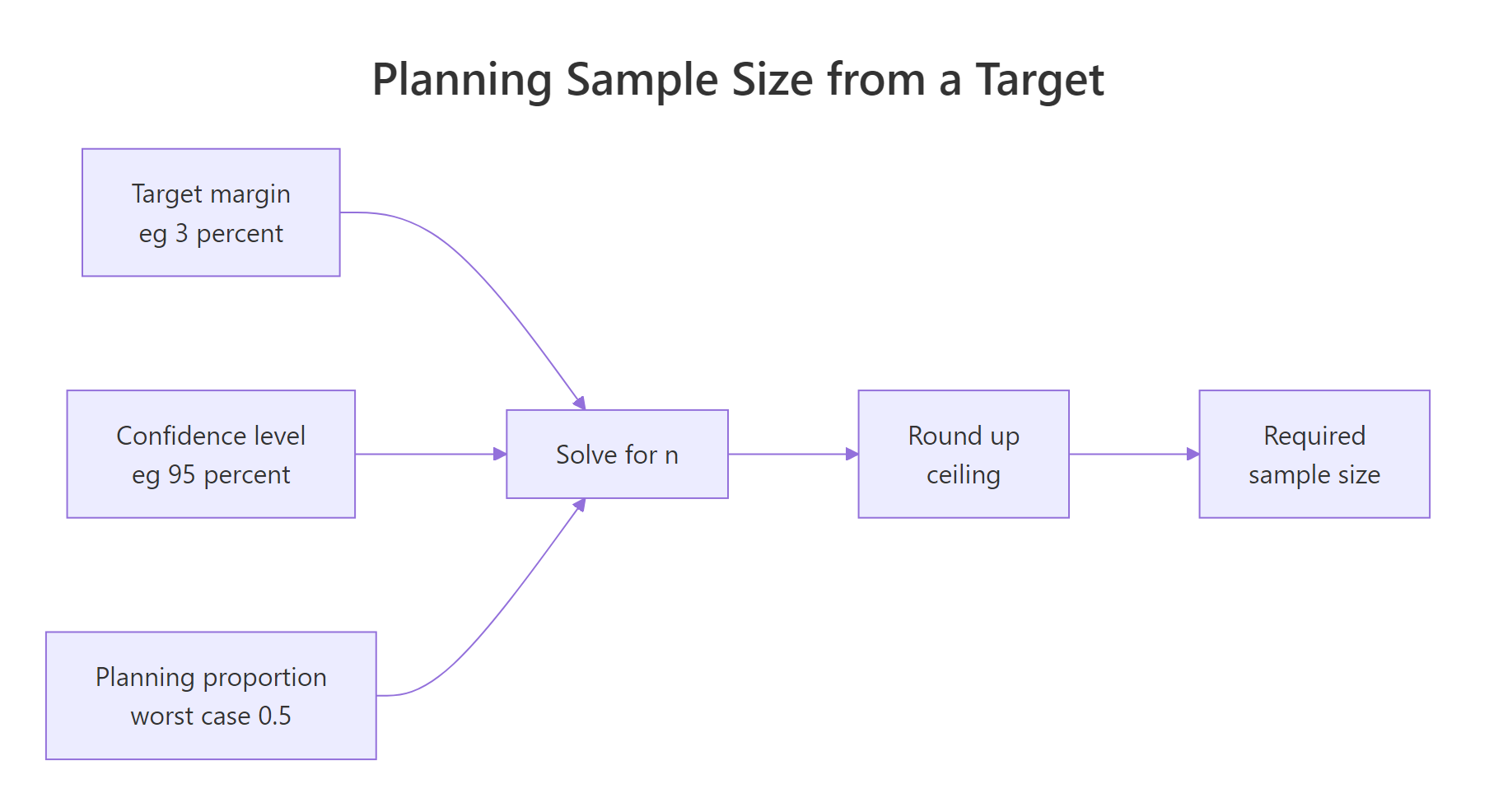
Figure 3: Planning a sample size inverts the margin-of-error formula and rounds up.
Try it: A less demanding survey only needs a 5-point margin of error at 95% confidence. Plan its worst-case sample size.
Click to reveal solution
Explanation: Relaxing the target from 3 points to 5 points drops the required sample from 1,068 to just 385. Because precision costs the square of itself, a slightly looser target saves an enormous amount of fieldwork.
What about the margin of error for a mean (not a proportion)?
Not every estimate is a percentage. Often you want an average: mean household income, mean response time, mean temperature. The margin of error works the same way, a critical value times a standard error, but two things change. The spread now comes from the standard deviation of the data, and because we rarely know the true spread and have to estimate it from the sample, we use a slightly larger multiplier from the t distribution instead of the normal z, which widens the interval a touch to account for that extra uncertainty.
$$\text{MoE}_{\text{mean}} = t^* \times \frac{s}{\sqrt{n}}$$
Let us compute the margin of error for the average miles-per-gallon in R's built-in mtcars data. R gives us the t critical value with qt(), which needs the degrees of freedom, one less than the sample size.
The average fuel economy across these 32 cars is 20.09 mpg, with a margin of error of 2.17 mpg. So a fair report is "about 20 mpg, give or take 2.2," with the true average for the wider population of cars this sample represents landing somewhere between 17.9 and 22.3 mpg. The logic is identical to the poll; only the ingredients differ.
You do not have to assemble this by hand. R's t.test() builds the same confidence interval for you, and the margin of error is just half of its width. This is a handy way to check your work.
The bounds match to the decimal, and the half-width is 2.173, exactly the margin of error we computed by hand. Planning a sample size for a mean uses the same inversion as before, but it needs one input you have to supply yourself: a guess for the spread, written $\sigma$. You usually get it from a small pilot study or from past data. The planning formula uses the normal $z^$ rather than the $t^$ from above, because the degrees of freedom depend on $n$, the very number we are trying to find.
$$n = \left(\frac{z^* \, \sigma}{E}\right)^2$$
Using the observed mpg spread as our pilot estimate, pinning the average down to within 1 mpg would take about 140 cars, far more than the 32 we have. That is the honest cost of tightening a margin of error from 2.2 down to 1.
Try it: Estimate the margin of error for the average Wind speed in R's built-in airquality data at 95% confidence.
Click to reveal solution
Explanation: With 153 wind readings, the mean is precise to within about 0.56 mph. The larger sample size here delivers a tighter margin of error than the 32-car mpg example, exactly as the square-root rule predicts.
Does the margin of error formula actually work? (simulation check)
The formula is tidy, but should you trust it? A 95% margin of error makes a testable promise: if many researchers each drew their own sample and each built an interval of estimate plus-or-minus the margin of error, about 95% of those intervals should contain the true value. We can check that promise directly by building a world where we know the truth, then sampling from it thousands of times and counting the hits.
Let us create a population where exactly 60% are supporters, draw 5,000 separate samples of 800 people, and for each one test whether the interval captured the true 60%.
Exactly 95%. Out of 5,000 samples, each blind to the truth, 95% built an interval that successfully bracketed the real 60%. Each person in a sample is coded 1 for a supporter and 0 for everyone else, so mean(s) is simply that sample's proportion of supporters. The replicate() function just repeated the "draw 800 people, build an interval, did it capture the truth" experiment 5,000 times and stored the yes-or-no answer each time. Averaging those yes-or-no results gives the capture rate, and it landed right on the promised 95%. The formula is not a rough approximation here; it delivers precisely what it advertises.
Try it: Rerun the check with a 90% margin of error by swapping the multiplier from 1.96 to 1.645. The capture rate should drop to about 90%.
Click to reveal solution
Explanation: The narrower 90% interval captured the truth only about 91% of the time, close to its promised 90%. A smaller margin of error catches the truth less often. That is the exact trade you make every time you lower your confidence level.
When should I use the finite population correction?
Every formula so far quietly assumed your population is effectively infinite, or at least so large that your sample is a tiny sliver of it. That is fine for polling a country. But when your sample is a big chunk of a small, closed group, say you survey 340 of a club's 594 members, you actually know more than the standard formula credits you for, and your true margin of error is smaller. The fix is the finite population correction, a shrinking factor you multiply onto the margin of error.
$$\text{FPC} = \sqrt{\frac{N-n}{N-1}}$$
Where $N$ is the population size and $n$ is the sample size. Let us reproduce a real case: a pollster who sampled 340 of 594 legislators and reported a 3-point margin.
Ignoring the correction, the margin of error looks like 5.3 points. But because 340 people is well over half of all 594, the correction pulls it down to 3.5 points. That is why the pollster could honestly claim a roughly 3-point margin: sampling most of a small population is genuinely more precise than sampling the same number from a huge one. The same logic feeds back into planning. When the population is finite, you can shave the required sample size too.
For a 3-point margin, the infinite-population formula demands 1,068 people. But if your entire population is only 8,000, the correction trims that to 943, a real saving. The smaller the population relative to your sample, the bigger the discount.
Try it: You plan to survey members of a 2,000-person organization and want a 3-point margin of error. Use the finite-population planner to find the sample size.
Click to reveal solution
Explanation: Against a population of only 2,000, the required sample falls from 1,068 to 697. Because your sample is now a sizable fraction of everyone, each person you add tells you proportionally more about the whole group.
A Complete Example: Planning a Customer Satisfaction Survey
Let us run the full pipeline end to end. Suppose you manage a subscription product with 8,000 customers, and you want to estimate the share who are satisfied to within 4 points at 95% confidence. You have no prior estimate, so you plan for the worst case of 0.5, and because 8,000 is a finite, closed population, you apply the correction.
The infinite-population formula asks for 601 responses; the finite correction trims it to 560 given your 8,000 customers. So your plan is to collect 560 completed surveys. Now fast-forward: you run the survey, 560 people respond, and 68% say they are satisfied. Let us simulate those responses and compute the margin of error you can actually report.
The report is now straightforward to write: 68.2% of customers are satisfied, with a margin of error of 3.7 points, so the true satisfaction rate across all 8,000 customers is very likely between 64.5% and 71.9%. Notice the realized margin of error, 3.7 points, came in comfortably under your 4-point target, because the satisfied share landed away from the worst-case 0.5. You planned for the hardest case and got a slightly better result than promised, which is exactly how conservative planning is supposed to feel.
Practice Exercises
These combine several ideas from the guide. Each uses fresh variable names so it will not disturb the functions and data from earlier. Try each before opening the solution.
Exercise 1: Worst case versus a known proportion
A pollster wants a 2-point margin of error at 95% confidence. Compute the required sample size two ways: the worst-case plan with p = 0.5, and a plan that uses prior knowledge that the proportion is near 0.2. By how much does the prior knowledge cut the sample?
Click to reveal solution
Explanation: Knowing the proportion is near 0.2 cuts the required sample from 2,401 to 1,537, a saving of over 800 people. Lopsided proportions vary less, so they are cheaper to measure. When you have credible prior information, use it.
Exercise 2: Is the current sample big enough for a mean?
You want to estimate the average mpg in mtcars to within 1.5 mpg at 95% confidence. Using the observed standard deviation as your pilot estimate, how many cars would you need? Then compute the margin of error the current 32 cars actually deliver, and decide whether 32 is enough.
Click to reveal solution
Explanation: Reaching a 1.5 mpg margin would take about 63 cars, but the current 32 cars only deliver a margin of 2.17 mpg. So 32 is not enough for that target; you would need to roughly double the sample. The planner tells you this before you commit, not after.
Exercise 3: How much does a finite population save?
A club has 500 members and you want to estimate a proportion to within 4 points at 95% confidence. Compute the sample size ignoring the finite population, then with the finite population correction, and report how many surveys you save.
Click to reveal solution
Explanation: Because 500 is a small population, the correction more than halves the required sample, from 601 down to 274, saving 327 surveys. Whenever your target sample is a large fraction of the whole group, checking the finite correction can save real time and money.
Frequently Asked Questions
Is the margin of error the same as the standard error?
No, but they are close relatives. The standard error is the typical bounce of your estimate from sample to sample. The margin of error is that standard error multiplied by a critical value, so it also carries your confidence level. In short, the margin of error is a scaled-up standard error tuned to how sure you want to be.
What confidence level does a margin of error assume?
By convention, 95%, unless stated otherwise. That is where the famous 1.96 multiplier comes from. If a report gives a margin of error without naming a confidence level, it is almost always 95%. Changing the level changes the multiplier: 1.645 for 90%, 2.576 for 99%.
Why do national polls usually report a 3-point margin of error?
Because a 3-point margin at 95% confidence needs about 1,068 people, and roughly a thousand respondents is an affordable, practical sample. Tightening to 2 points would require more than 2,400 people, and thanks to the square-root rule, that extra precision rarely justifies the added cost.
Does a bigger sample always shrink the margin of error?
Yes, but with sharply diminishing returns. Because precision improves with the square root of the sample size, you need four times the data to halve the margin of error. One caveat: a bigger sample cannot fix a biased one. If your sampling method systematically misses people, more data just gives you a more confident wrong answer.
What is different about the margin of error for a mean?
Two things. The spread comes from the standard deviation of the data rather than from a proportion, and because you estimate that spread from the sample, you use a t critical value from qt() instead of the normal z. With more than about 30 observations the two multipliers are nearly identical.
Is planning for a margin of error the same as a power calculation?
No. Sizing a sample for a target margin of error is about making an estimate precise. A power calculation sizes a sample to reliably detect an effect or difference in a hypothesis test. They answer the same "how many do I need" question with different goals, so the numbers can differ.
Summary
The margin of error is the disciplined plus-or-minus on any estimate built from a sample. Compute it, and your number comes with an honest statement of how far it might sit from the truth. Plan around it, and you know how big a sample your question actually requires. Here are the ideas to carry forward.
| Idea | Plain meaning |
|---|---|
| Margin of error | Half the width of a confidence interval, the plus-or-minus around your estimate. |
| The formula | A critical value times a standard error; the two levers are confidence and sample size. |
| Square-root rule | Precision improves with the square root of the sample; four times the data to halve the margin. |
| Planning a proportion | Invert the formula and round up; use p = 0.5 as the worst case when you have no prior. |
| Margin for a mean | Use a t critical value and the data's standard deviation; planning needs a pilot estimate of spread. |
| Finite population correction | Shrinks the margin when your sample is a big fraction of a small population. |
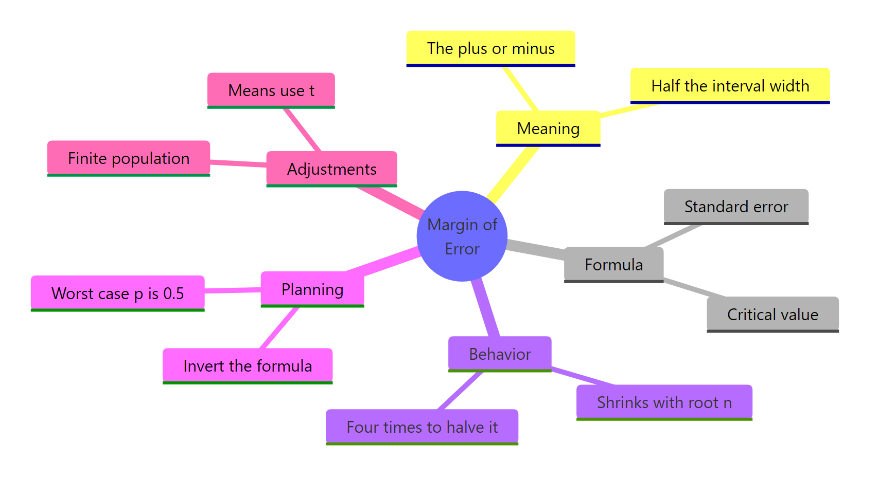
Figure 4: The whole margin-of-error and sample-size picture on one page.
You now have a complete, runnable toolkit: compute a margin of error for a percentage or an average, plan the sample size to hit any target precision, correct for a finite population, and verify by simulation that the formula keeps its promise. Every survey you read or design will make more sense for it.
References
- R Core Team. An Introduction to R, probability distributions and
qnorm/qt. Link - Diez, D., Barr, C., Cetinkaya-Rundel, M. OpenIntro Statistics, 4th Edition. Confidence intervals and sample size. Link
- Cochran, W. G. Sampling Techniques, 3rd Edition. Wiley (1977). Sample size and the finite population correction. Link
- R Tutor. Sampling Size of Population Proportion. Link
- R-bloggers. Understanding Margin of Error for Small Populations. Link
- Scribbr. How to Calculate Margin of Error. Link
- Wikipedia. Margin of error. Link
Continue Learning
- Confidence Intervals in R is the full interval that the margin of error is half of, with the same critical-value machinery.
- Sample Size Planning in R covers sizing a sample to detect an effect, the power-based companion to the precision-based planning here.
- Statistical Power Analysis in R shows how to size studies for hypothesis tests, the other half of the "how many do I need" question.