Zero-Inflated and Hurdle Models in R
Zero-inflated and hurdle models are count models for data that piles up far more zeros than an ordinary Poisson model can explain. Both split the problem into two parts: one part decides whether a zero happens at all, and a second part explains the size of the counts. This guide builds both models from one small fishing dataset in R, shows how to read each half, and gives you a clear rule for choosing between them. It uses base R plus the pscl package, and every block runs right here in your browser.
Why do too many zeros break an ordinary Poisson model?
A Poisson model is the usual first choice for counting things, like fish caught, doctor visits, or insurance claims. It carries one strong assumption baked in: the average count and the spread of counts are the same number, which also fixes how many zeros it expects to see. When real data has far more zeros than the average can account for, the Poisson fit is wrong across the board, not just on the zeros. Let's build a small dataset and watch that happen.
We will simulate 250 groups of visitors at a park. Each group has a size, a number of children, and a flag for whether they brought a camper. We deliberately build the fish counts from two hidden stories so we know the truth: some groups never fish at all, and the groups that do fish catch a Poisson number of fish.
Each row is one group and the fish column is what we want to model. Notice row 4 caught zero fish while row 6 caught fifteen. That mix of many zeros and a few large counts is the signature of the data we care about here.
How common are the zeros? Let's just ask.
Almost half the groups, 45.6 percent, caught no fish. On its own that number means nothing, because a Poisson process can produce plenty of zeros too. The real question is whether it produces this many zeros. To answer that, we fit a plain Poisson model and ask it how many zeros it would expect.
Here is the problem in one line. We saw 114 zeros, but the fitted Poisson model expected only about 51. It is off by more than sixty zeros. The model simply has no way to make that many zeros while also explaining the groups that caught ten or fifteen fish.
There is a second warning sign hiding in the spread of the counts. A Poisson variable has its variance equal to its mean, so let's compare them.
The variance, 15.85, is almost six times the mean of 2.74. Data that is far more spread out than its average is called overdispersed, and excess zeros are one of the most common causes of it. Both signals point the same way: this is not a job for plain Poisson.
So where do all those zeros come from? It helps to see that a zero can arrive by two very different routes.
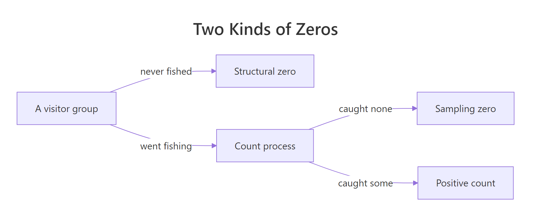
Figure 1: A zero can be structural (the group never fished) or a sampling zero (they fished but caught nothing).
Try it: The Poisson model could not explain all the zeros we saw. Compute how many observed zeros it failed to account for, using the two objects from the block above.
Click to reveal solution
Explanation: About 63 of the 114 zeros are extra zeros that a Poisson model cannot produce. That gap is exactly the hole the models in this guide are built to fill.
What is the real difference between zero-inflated and hurdle models?
Both models attach a second, smaller model to the count model, and that second model is in charge of the zeros. The difference is a subtle but important disagreement about where zeros are allowed to come from. Get this idea first and the R code afterwards will feel obvious.
A zero-inflated model says zeros come from two places at once. There is a hidden on/off switch that turns some observations into guaranteed "always zero" cases (the structural zeros), and separately the ordinary count process can also land on zero by chance (the sampling zeros). The zeros in your data are a blend of both.
A hurdle model tells a cleaner story. There is a single gate, or hurdle. You are either a zero or you clear the hurdle and become a positive count, and one binary model decides which. Once you clear the hurdle, a special count model that can never produce a zero explains how high you go. In a hurdle model, all zeros come from the gate, never from the count part.
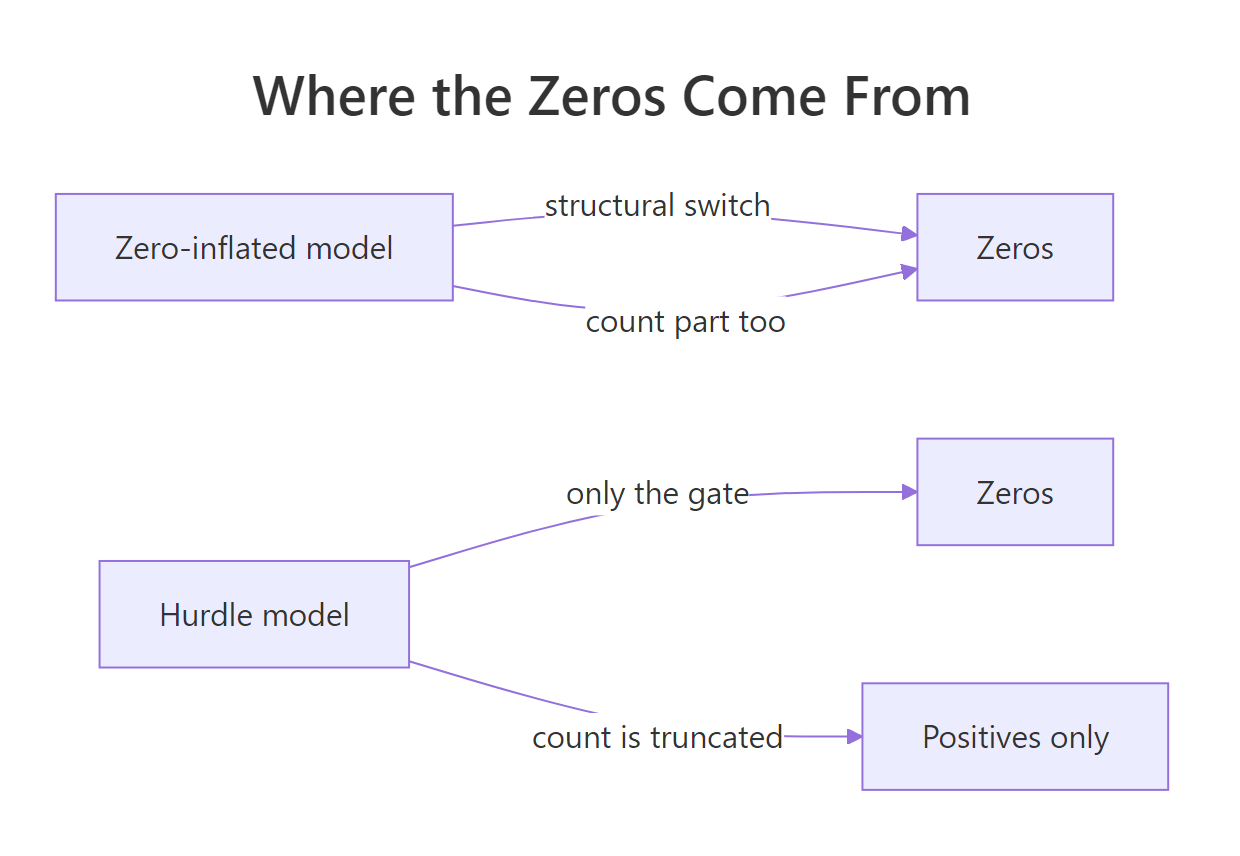
Figure 2: In a zero-inflated model both parts can make zeros; in a hurdle model only the gate does.
Here is the same contrast as a quick reference.
| Question | Zero-inflated | Hurdle |
|---|---|---|
| Where do zeros come from? | A switch plus the count model | The gate only |
| Can the count part make a zero? | Yes | No, it is truncated at 1 |
| Natural reading of the zero part | Chance of an always-zero case | Chance of clearing the hurdle |
| Good fit when | Zeros are a mix of two sources | Zero versus positive is a real threshold |
To see why children matter so much in our data, let's cross-tabulate the number of children against whether a group caught anything.
The pattern is stark. Among groups with no children, most caught something (72 of 101). Among groups with three children, almost none did (2 of 13). Children are pushing groups into the zero state, which is exactly the kind of predictor the zero part of these models is designed to hold.
fish ~ persons + camper | child. The left side models the counts and the right side models the zeros, and you can give each side a different set of predictors.Try it: Children clearly drive the zeros. Check whether the camper flag shows the same kind of split by making the same table for camper instead of child.
Click to reveal solution
Explanation: The camper split is mild (roughly half caught fish either way), so camper is a weak predictor of the zero state compared to children. That is a hint we should let children drive the zero part and let camper drive the count part.
How do you fit a zero-inflated Poisson model in R?
The zeroinfl() function from the pscl package fits a zero-inflated model in one call. We will let group size and the camper flag drive the count of fish, and let the number of children drive the chance of being a structural zero. That is the count ~ ... | zero formula from the last section.
The summary prints two blocks of coefficients because you fit two models at once. Read them one at a time.
The top block, the count model, is an ordinary Poisson regression on the log scale. The persons coefficient of 0.609 is positive and highly significant, so bigger groups catch more fish. The camper coefficient of 0.814 says camper groups catch more too. These are the numbers for groups that are actually in the fishing process.
The bottom block, the zero-inflation model, is a logistic regression that predicts the probability of being a structural zero, that is, an "always zero" group. The child coefficient is positive, 0.895, so more children raises the chance that a group is one of those never-fishing cases. This is where the excess zeros are coming from, and the model recovers the story we built into the data.
The log scale is hard to feel, so exponentiate the coefficients to get numbers you can talk about.
Now the count part reads as rate ratios. Each extra person multiplies the expected catch by about 1.84, and having a camper multiplies it by about 2.26, holding the other predictor fixed. The zero part reads as odds ratios: each additional child multiplies the odds of being a structural zero by about 2.45. A family with more kids is far more likely to be a group that was never going to fish.
If you like seeing the mechanics, the zero-inflated Poisson splits the probability of each outcome like this. Skip to the next section if formulas are not your thing, since the code above already tells the whole story.
$$P(Y = 0) = \pi + (1 - \pi)\,e^{-\lambda}$$
$$P(Y = k) = (1 - \pi)\,\frac{\lambda^{k} e^{-\lambda}}{k!}, \quad k = 1, 2, 3, \dots$$
Where:
- $\pi$ = the probability of being a structural zero (from the logistic zero part)
- $\lambda$ = the Poisson rate for the count part
- The zero row has two pieces: the structural zeros ($\pi$) plus the ordinary Poisson zeros $(1 - \pi)e^{-\lambda}$
Try it: Pull the rate ratio for persons out of the exponentiated coefficients. The name you want is count_persons, not count_camper.
Click to reveal solution
Explanation: Each extra person in a fishing group multiplies the expected number of fish by about 1.84, all else equal.
How do you fit a hurdle model in R?
Fitting a hurdle model uses the same formula and the same package. Only the function name changes, from zeroinfl() to hurdle(). The story it tells about the zeros, though, flips around, so read the zero part carefully.
The count block on top is almost the same as before, with one label change: it is now a truncated Poisson, meaning a Poisson that is not allowed to be zero. That truncation is what lets the gate own all the zeros.
The zero block at the bottom is where the reading flips. In a hurdle model this part predicts the probability of clearing the hurdle, that is, catching at least one fish. The child coefficient is now negative, -0.873, which says more children lowers the chance of catching anything. Compare that to the zero-inflated fit, where the child coefficient was positive because it predicted the opposite event, the chance of being an always-zero case.
The count ratios tell the same story as the zero-inflated model: more persons and a camper both raise the catch. The zero-part ratio for child is now 0.42, meaning each extra child multiplies the odds of catching any fish by about 0.42, so it cuts those odds by more than half. The same predictor points the opposite way here, because the two models are describing opposite events.
For completeness, the hurdle model factors each probability like this. Feel free to skip it, since the fitted output above is all you need to use the model.
$$P(Y = 0) = 1 - p$$
$$P(Y = k) = p \cdot \frac{\lambda^{k} e^{-\lambda}}{(1 - e^{-\lambda})\,k!}, \quad k = 1, 2, 3, \dots$$
Where:
- $p$ = the probability of clearing the hurdle (from the logistic zero part)
- $\lambda$ = the rate of the truncated Poisson count part
- Dividing by $(1 - e^{-\lambda})$ rescales the Poisson so it never returns a zero
Try it: Using the hurdle model, find the probability that a group catches at least one fish when it has no children versus two children. The helper below sets up the two groups for you.
Click to reveal solution
Explanation: A childless group clears the hurdle about 72 percent of the time, but a group with two children only about 31 percent of the time. Children more than halve the chance of catching anything.
How do you handle overdispersion with negative binomial versions?
Sometimes the counts that clear the hurdle are still more spread out than a Poisson allows. The fix is the same one you would use for any count model: swap the Poisson for a negative binomial, which adds a dispersion parameter that lets the variance grow past the mean. Both zeroinfl() and hurdle() accept dist = "negbin".
That theta is the negative binomial's dispersion parameter, and a very large value is informative. As theta grows toward infinity the negative binomial becomes identical to a Poisson. A theta in the hundreds of thousands means the model found no leftover overdispersion to absorb: once the excess zeros were handled, there was nothing extra for the negative binomial to do.
The clean way to confirm that is to line all five models up by AIC, a score where lower means a better trade-off between fit and complexity.
The plain Poisson is far behind at 1275.8, which confirms it was the wrong model. The two-part models all cluster around 825 to 832, a massive improvement. The negative binomial versions (zinb and hnb) score slightly worse than their Poisson twins, because they spend an extra parameter on dispersion that this data does not need. Here the plain hurdle Poisson (hp) wins.
Try it: Read the AIC of the negative binomial hurdle model, hnb, and compare it in your head to the plain hurdle Poisson's 822.5.
Click to reveal solution
Explanation: At 824.5, the negative binomial hurdle scores about two points worse than the plain hurdle Poisson at 822.5. The extra dispersion parameter is not earning its keep on this data.
How do you choose between the models?
AIC gives you a single number, but you should never lean on one number alone. A second, more honest check for count data is to ask each model how many zeros it predicts and compare that to the 114 zeros you actually saw. A model built for excess zeros should get the zero count roughly right.
The Poisson predicts only 51 zeros against 114 observed, a failure you already knew about. The zero-inflated models land close, at about 117. The hurdle model matches it exactly at 114, and that is not luck. A hurdle model reproduces the observed number of zeros by construction, because its gate is fit directly to the zero-versus-positive split. That reliability is one reason hurdle models are popular.
You may have read about the Vuong test for comparing these models. Treat it with caution: its use for comparing zero-inflated against standard models has been criticized and is no longer recommended by many authors, including the pscl maintainers. AIC together with the predicted-zeros check is a more dependable pairing.
That leaves the real decision, which is about your data's story rather than any single statistic.
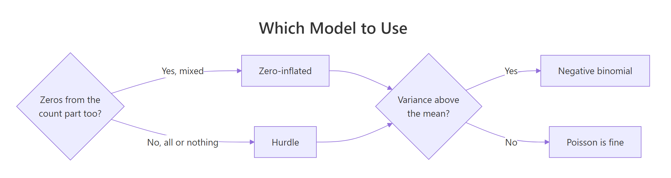
Figure 3: A quick decision guide for choosing a count model when zeros pile up.
Use this to guide the choice:
- Can a zero come from the counting process itself? If a subject who is "in" the process could still record a zero by chance, a zero-inflated model fits the story. If a zero always means the subject never entered the process, a hurdle model fits better.
- Is there a clean threshold between zero and positive? Cases like "signed up versus never signed up" are natural hurdles. Cases where zeros and low counts blur together lean zero-inflated.
- Is the variance still above the mean after fitting? If the leftover spread is large, switch that model to its negative binomial form. If not, keep the simpler Poisson version.
Try it: Let R pick the winner for you by finding which of the five models has the lowest AIC.
Click to reveal solution
Explanation: The plain hurdle Poisson (hp) has the lowest AIC, matching what the predicted-zeros check told us.
How do you make predictions from the fitted model?
A fitted model is most useful when it makes predictions for new cases. The predict() function understands several type values, and each one answers a different question. The most useful are "response" for the expected count, "zero" for the probability of the zero state, and "prob" for the full probability of each possible count.
Let's predict for a new group: three people, no children, with a camper.
The zero-inflated model expects this group to catch about 5.6 fish on average, and it puts the probability that they are a never-fishing structural zero at about 24 percent. The expected count of 5.6 already blends both parts: it is the count-model rate scaled down by the chance of being an always-zero group.
The hurdle model answers the same two questions with its own wording.
The hurdle model expects about 5.3 fish and gives this group a 28 percent chance of catching nothing. The two models land close on the expected count, which is reassuring, and they express the zero side in their own natural language: a structural-zero probability for zero-inflated, a plain probability of zero for hurdle.
Try it: Predict the expected catch for a large group with children: four people, two children, and a camper. Use the zero-inflated model.
Click to reveal solution
Explanation: Even though this group is larger, the two children pull the expected catch down to about 4.7 fish, because children raise the chance of the structural-zero state.
Practice Exercises
These exercises combine several ideas from the guide. Try each one before opening the solution. They use their own variable names so they will not disturb the models you fit above.
Exercise 1: Diagnose and fit on new data
A subscription business counts monthly purchases for 300 customers and suspects that many customers are window-shoppers who never buy. The starter builds the data. Your job is to confirm the excess-zero problem by comparing observed zeros to what a Poisson expects, then fit a zero-inflated Poisson and check whether tenure significantly predicts the zero state.
Click to reveal solution
Explanation: The Poisson expects only about 69 zeros but the data has 104, so the excess is real. In the zero part, tenure has a strongly significant negative coefficient, meaning longer-tenured customers are much less likely to be in the never-buying state.
Exercise 2: Does a predictor belong in the zero part?
Using the fishing data, you already fit a zero-inflated Poisson with only child in the zero part. Test whether adding persons to the zero part improves the model. Fit both, compare their AIC, and look at whether the new coefficient is significant.
Click to reveal solution
Explanation: Adding persons to the zero part raises the AIC from 830.3 to 830.6, so it makes the model slightly worse, and the new coefficient is not significant (p = 0.20). Keep persons in the count part where it belongs and leave the zero part to child.
Exercise 3: Interpret a hurdle model by hand
Confirm that you can reproduce predict() from the raw coefficients of the hurdle model hp. Compute the rate ratio for camper in the count part, then compute the probability that a group with one child clears the hurdle, and check it against predict().
Click to reveal solution
Explanation: Having a camper multiplies the expected catch by about 2.37. A group with one child clears the hurdle about 52 percent of the time, and the by-hand calculation matches predict() exactly, which shows the zero part really is just a logistic regression.
Frequently Asked Questions
When should I use a zero-inflated model instead of a hurdle model?
Use a zero-inflated model when a zero can come from two sources: subjects who are never at risk plus subjects who are at risk but happened to score zero. Use a hurdle model when every zero means the subject never crossed a threshold, so zero and positive are two clean states. When the two fit almost equally well, pick the one whose story matches your data.
What does the vertical bar in the formula mean?
The bar separates the two models. Everything before it, as in fish ~ persons + camper, are the predictors for the count part. Everything after it, as in | child, are the predictors for the zero part. You can use different predictors on each side, and if you leave the right side off, both parts share the same predictors.
Why did the negative binomial version not improve my model?
Excess zeros and overdispersion look similar in raw data, and both inflate the variance. Once a zero-inflated or hurdle model explains the zeros directly, the leftover overdispersion can vanish, so the negative binomial's extra parameter has nothing to absorb. A theta that shoots up to a huge value is the sign that the negative binomial has collapsed back to a Poisson.
Can I use the Vuong test to compare these models?
You can compute it, but treat it carefully. Its use for testing zero-inflated models against standard count models has been criticized and is no longer recommended by many statisticians, including the pscl authors. Comparing AIC and checking each model's predicted number of zeros against the observed count is a more reliable approach.
Do these models work in local RStudio the same way?
Yes. Everything in this guide uses base R plus the pscl and MASS packages, which are standard CRAN packages. The same code runs unchanged in RStudio; install pscl once with install.packages("pscl") and you are set.
Summary
Zero-inflated and hurdle models handle count data with more zeros than a Poisson can explain by splitting the process into a zero part and a count part. Diagnose the problem first by comparing observed zeros to Poisson-expected zeros, then fit both models, then choose with AIC and a predicted-zeros check.
| Model | What it assumes about zeros | R call | Reach for it when | |
|---|---|---|---|---|
| Poisson | Zeros come only from the count process | glm(..., family = poisson) |
Mean and variance are close, zeros are not excessive | |
| Zero-inflated | A switch adds structural zeros on top of count zeros | `zeroinfl(y ~ x | z)` | Zeros mix two sources: never-at-risk plus at-risk-but-zero |
| Hurdle | One gate decides zero versus positive; counts are truncated | `hurdle(y ~ x | z)` | Zero versus positive is a real threshold |
| Negative binomial variants | Same as above, plus extra spread in the counts | dist = "negbin" |
Variance is still above the mean after fitting |
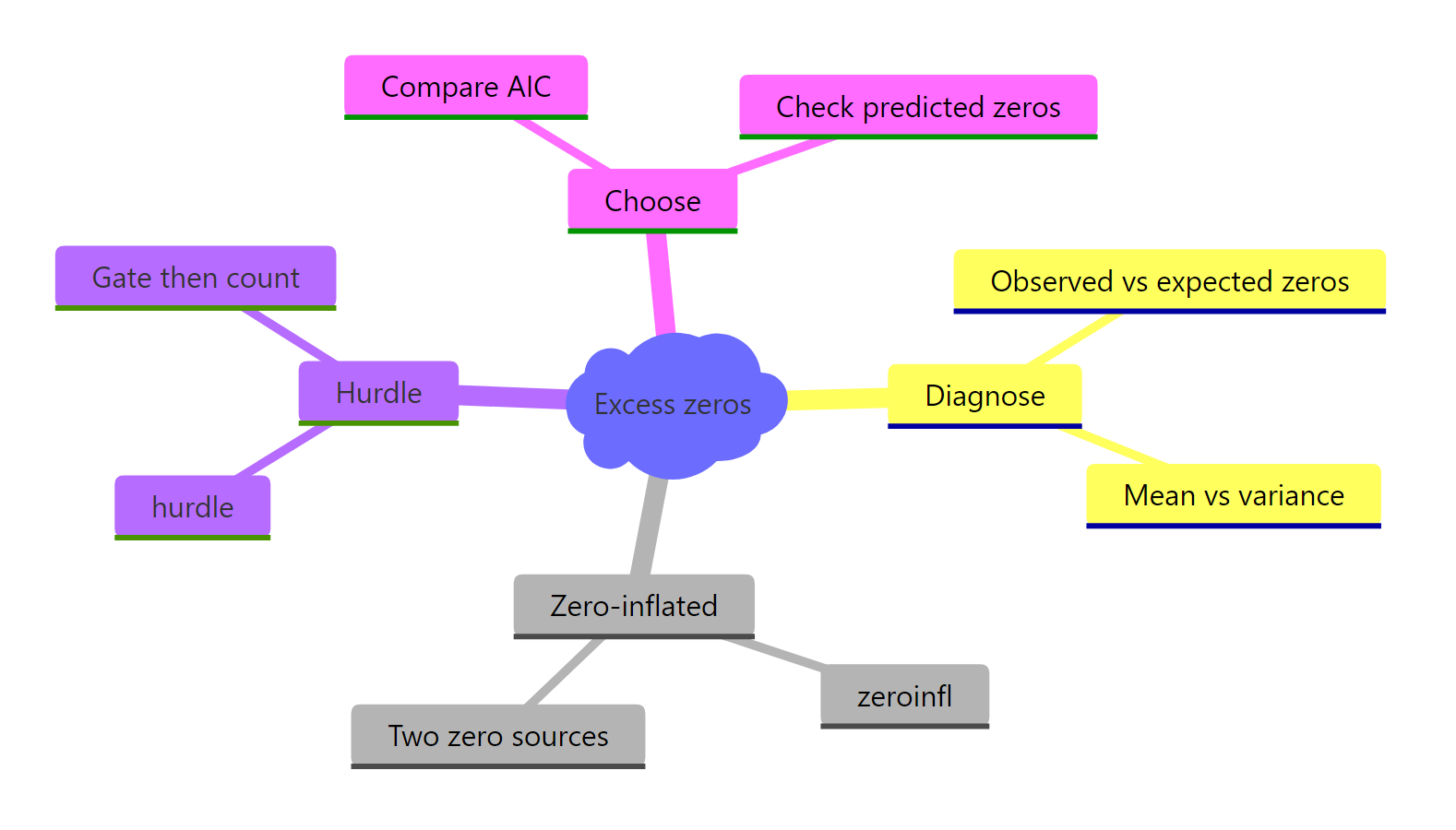
Figure 4: The whole workflow, from diagnosing the zeros to choosing a model.
The biggest ideas to carry with you: excess zeros break a Poisson model in a way you can measure, the vertical-bar formula fits two models at once, and the sign of the zero part flips between zero-inflated and hurdle because they model opposite events.
References
- Zeileis, A., Kleiber, C., & Jackman, S. (2008). Regression Models for Count Data in R. Journal of Statistical Software, 27(8). Link - the canonical paper behind
pscl, with the theory and R syntax for bothzeroinfl()andhurdle(). - pscl package reference:
zeroinfl()andhurdle(). Link - the official function docs, listing every argument used in this guide. - UCLA OARC Statistical Consulting. Zero-Inflated Poisson Regression. Link - a worked ZIP walkthrough in R whose approach closely mirrors this one.
- Cameron, A. C., & Trivedi, P. K. (2013). Regression Analysis of Count Data, 2nd Edition. Cambridge University Press. - the standard textbook treatment of count models, excess zeros, and overdispersion.
- Venables, W. N., & Ripley, B. D. (2002). Modern Applied Statistics with S (MASS), 4th Edition. Springer. Link - background on the negative binomial machinery that the
dist = "negbin"variants rely on. - Kleiber, C., & Zeileis, A. (2008). Applied Econometrics with R. Springer. Link - chapter-length examples of count-data models using the same R tooling.
- Feng, C. X. (2021). A comparison of zero-inflated and hurdle models for modeling zero-inflated count data. Journal of Statistical Distributions and Applications, 8(8). Link - a recent, direct comparison of the two model families to guide your choice.
Continue Learning
- Poisson and Negative Binomial Regression in R - the base count models that these two-part models extend.
- Offsets and Exposure in Poisson Models in R - turn raw counts into rates when groups are observed for different lengths of time.
- How to Read Logistic Regression Output in R - a deeper look at reading the logistic half that powers the zero part of both models.