Mixed Model Inference in R: p-Values and Bootstrap
Fit a mixed model with lme4 and you get estimates, standard errors, and t-values, but no p-value column. That is deliberate. This tutorial walks through every honest way to test a fixed effect in R: the t-as-z shortcut, the likelihood ratio test, the Satterthwaite and Kenward-Roger degrees-of-freedom methods, and the parametric bootstrap, all with runnable code and real output.
We use the built-in sleepstudy data throughout, and base our work on a model you may already know how to fit. If the fitting step is new to you, read Random Intercepts and Slopes with lme4 first, then come back here for the inference.
Why does lme4 leave the p-value column blank?
Here is the situation that sends most people searching for answers. You fit a mixed model, ask for the summary, and the fixed-effects table has a t value column but no p-value next to it. Let's reproduce that with the classic sleepstudy experiment, where 18 subjects had their reaction time measured over 10 days of sleep restriction.
The model below says reaction time changes with Days, and it lets each subject have their own baseline and their own rate of slowing down. That per-subject wiggle room is the random-effects part, written (Days | Subject).
Read that table one column at a time. Estimate says reaction time starts near 251 ms and rises about 10.5 ms for each extra day of sleep loss. Std. Error is the uncertainty in each estimate. t value is just the estimate divided by its standard error, so 10.467 / 1.546 gives 6.771. What is missing is the final column you get from lm(): the p-value.
This is not a bug. To turn a t-value into a p-value you need a reference distribution, and that distribution needs a "denominator degrees of freedom" number that says how much independent information the data really carry. In an ordinary regression that number is simple. In a mixed model the observations are not independent (measurements from the same subject are correlated), so the effective degrees of freedom sit somewhere between "number of subjects" and "number of rows", and there is no exact formula for where.
Try it: Pull just the Days row out of the fixed-effects table, keeping only its estimate and standard error.
Click to reveal solution
Explanation: coef(summary(fm)) returns a plain matrix, so you can index it with ["Days", c("Estimate", "Std. Error")] exactly like any other matrix.
Can you read significance straight off the t-value?
Yes, roughly, and this is the fastest sanity check you can do. When a study has plenty of data, the t-value behaves almost like a z-value from a standard normal curve. A z of about 2 marks the 5% two-sided cutoff, so the rule of thumb is simple: if the absolute t-value is bigger than 2, the effect is probably significant at the 0.05 level.
Our Days t-value is 6.771, which is far past 2, so we already expect a tiny p-value. Let's make that concrete by treating the t-value as a z-value and reading the two-sided tail probability off the normal curve.
pnorm(abs(t_days), lower.tail = FALSE) gives the probability of seeing a z at least this large in one tail, and doubling it covers both tails. The result, about 1.3e-11, is the "t-as-z" or Wald p-value. It says that if Days truly had no effect, a t-value this extreme would be almost impossible.
That answer is fine here because the effect is huge. The danger shows up when a t-value sits near the 2 boundary and the study has only a handful of groups.
Try it: Apply the rule of thumb directly. Write one line that returns TRUE when the Days effect clears the "absolute t greater than 2" bar.
Click to reveal solution
Explanation: abs() strips the sign so the test works for negative effects too, and the comparison returns a single TRUE or FALSE.
How do you get a real p-value with a likelihood ratio test?
The likelihood ratio test (LRT) gives you a p-value without ever needing to know the degrees of freedom of a t distribution. The idea is to compare two models: the full model that includes Days, and a null model that drops it. If dropping Days barely hurts the fit, the effect was not doing much. If it hurts a lot, Days matters.
"How well a model fits" is measured by its log-likelihood, and twice the gap in log-likelihood follows a known chi-squared curve:
$$D = 2\left(\ell_{\text{full}} - \ell_{\text{null}}\right) \sim \chi^2_{k}$$
Where:
- $\ell_{\text{full}}$ and $\ell_{\text{null}}$ are the maximized log-likelihoods of the two models
- $k$ is the number of parameters you removed (here, 1: the
Daysslope) - $D$ is the deviance difference, which the chi-squared curve turns into a p-value
There is one setup rule. For testing a fixed effect this way, both models must be fit by plain maximum likelihood, not the default REML (restricted maximum likelihood), so we pass REML = FALSE. Then anova() does the comparison.
The Chisq value of 23.537 is the deviance difference $D$, Df is 1 because we removed one parameter, and Pr(>Chisq) of 1.2e-06 is your p-value. Adding Days improves the fit far more than chance would allow, so the slope is real.
The LRT is trustworthy for fixed effects when your sample is not tiny. It is less reliable for testing whether a variance component is zero, because that hypothesis sits on the boundary of what is possible (a variance cannot go below zero), which makes the naive chi-squared p-value too large. We return to that boundary problem in the exercises.
Try it: You do not have to read the p-value off the printed table by eye. Pull it out of the anova() result directly.
Click to reveal solution
Explanation: The first row of the table is the null model (no test), so the p-value lives in the second row of the Pr(>Chisq) column.
How do you get p-values with Satterthwaite and Kenward-Roger degrees of freedom?
The likelihood ratio test sidesteps degrees of freedom, but many fields still want the familiar per-coefficient p-value in the summary table. Two methods estimate the missing denominator degrees of freedom so a t-test or F-test becomes possible: the Satterthwaite approximation and the Kenward-Roger approximation. Both try to answer "how much independent information does this effect really rest on?" with a fractional degrees-of-freedom number.
The lmerTest package adds these p-values to lmer output automatically, and the pbkrtest package supplies the Kenward-Roger machinery. These two packages are not part of the in-browser code sandbox, so run the blocks in this section in your own R or RStudio session. The output shown is the real result from R 4.6.0.
library(lmerTest)
fm_lt <- lmer(Reaction ~ Days + (Days | Subject), data = sleepstudy)
anova(fm_lt)
#> Type III Analysis of Variance Table with Satterthwaite's method
#>      Sum Sq Mean Sq NumDF DenDF F value    Pr(>F)
#> Days  30031   30031     1    17  45.853 3.264e-06 ***
Loading lmerTest and refitting gives an ANOVA table with a real p-value of 3.3e-06 for Days. The key number is DenDF, the estimated denominator degrees of freedom: 17, which is close to "18 subjects minus 1". That matches intuition, because the Days effect is learned mostly from how the 18 subjects differ, not from all 180 rows.
You can also see the per-coefficient version, which now carries a df and a Pr(>|t|) column that plain lme4 refused to print.
summary(fm_lt)$coefficients
#>             Estimate Std. Error       df   t value     Pr(>|t|)
#> (Intercept) 251.40510   6.824597 16.99973 36.838090 1.171558e-17
#> Days         10.46729   1.545790 16.99998  6.771481 3.263824e-06
The Kenward-Roger method is a more refined cousin that also adjusts the standard errors, and it is the safest choice for small samples. You request it by name.
anova(fm_lt, ddf = "Kenward-Roger")
#> Type III Analysis of Variance Table with Kenward-Roger's method
#>      Sum Sq Mean Sq NumDF DenDF F value    Pr(>F)
#> Days  30031   30031     1    17  45.853 3.264e-06 ***
For this balanced, well-behaved dataset Satterthwaite and Kenward-Roger agree exactly (both land on 17 degrees of freedom). They diverge on smaller or messier designs, where Kenward-Roger's extra correction tends to hold the false-positive rate closest to the advertised 5%.
Try it: The p-value above is just a t-test with a chosen degrees-of-freedom value. Reproduce the Satterthwaite p-value yourself using base R, the Days t-value of 6.7715, and the estimated 17 degrees of freedom.
Click to reveal solution
Explanation: This is exactly what lmerTest did internally: it plugged the estimated degrees of freedom into an ordinary t-distribution, which is why the result matches the table's 3.26e-06.
How do you turn estimates into confidence intervals?
A p-value tells you whether an effect differs from zero. A confidence interval tells you the plausible range for its size, which is usually the more useful thing to report. lme4 gives you three flavors through one function, confint(), and here we cover the two fast ones.
The quickest is the Wald interval, which assumes the estimate follows a symmetric bell curve and adds and subtracts a multiple of the standard error:
$$\hat{\beta} \pm z_{1-\alpha/2}\,\widehat{\text{SE}}(\hat{\beta})$$
Where $\hat{\beta}$ is the estimate, $\widehat{\text{SE}}$ is its standard error, and $z_{1-\alpha/2}$ is about 1.96 for a 95% interval. The parm = "beta_" argument restricts the output to the fixed effects.
The Days slope plausibly lies between 7.44 and 13.50 ms per day. Because the interval sits well above zero, this agrees with every p-value we have computed: the effect is clearly positive.
The Wald interval is fast but leans on that symmetry assumption. The profile interval drops the assumption by tracing how the likelihood actually changes as each parameter moves, so it can come out slightly asymmetric and is generally more accurate.
The profile interval for Days, 7.36 to 13.58, is a touch wider than the Wald one. For fixed effects in a healthy model the two usually agree closely, as they do here. The gap grows for variance parameters, where symmetry is a poor assumption and the profile interval is the one to trust.
Try it: Not every report wants 95%. Build a 90% Wald interval for the Days slope by setting the level argument.
Click to reveal solution
Explanation: A 90% interval is narrower than a 95% one because you are asking for less confidence, so the labels change to the 5% and 95% quantiles.
How does the parametric bootstrap give inference you can trust?
Every method so far leans on a mathematical approximation: the normal curve, the chi-squared curve, or an estimated degrees-of-freedom number. The parametric bootstrap replaces the approximation with brute force. The recipe is short: treat your fitted model as if it were the truth, simulate many fresh datasets from it, refit the model to each one, and watch how much the estimate bounces around. That spread is a direct, assumption-light picture of your uncertainty.
lme4 wires this straight into confint() with method = "boot". We set a seed so the random simulation is repeatable, and use a modest number of simulations to keep it quick.
The bootstrap interval for Days, 7.10 to 13.39, lands in the same neighborhood as the Wald and profile intervals. When all three roughly agree, you can be confident the approximations were safe. When the bootstrap disagrees, trust the bootstrap.
To really see what is happening, collect the individual simulated slopes with bootMer and look at their distribution. bootMer refits the model to each simulated dataset and records whatever statistic you ask for, which you supply as a function. Here that function is fixef(m)[["Days"]]: fixef() pulls the vector of fixed-effect estimates out of a fitted model, and [["Days"]] keeps the slope. bootMer returns an object whose $t component holds one recorded value per simulation, so boot_slope$t is the full set of 200 replicate slopes.
Taking the 2.5% and 97.5% quantiles of the 200 refitted slopes gives a 95% interval of 7.22 to 13.23, built entirely from simulation. Plotting the full set of replicates shows the bell-like spread the interval summarizes, with the two cutoffs marked.
The histogram is centered near the estimate of 10.5 and tapers off symmetrically, which is why the bootstrap and Wald intervals matched: for this model the sampling distribution really is close to normal.
The bootstrap can also produce a p-value for the whole Days effect, through PBmodcomp in the pbkrtest package. It runs the same full-versus-null comparison as the likelihood ratio test, but instead of trusting the chi-squared curve, it simulates the null world many times and counts how often chance alone beats your observed result.
library(pbkrtest)
set.seed(303)
PBmodcomp(fm_ml, null_ml, nsim = 100)
#> large : Reaction ~ Days + (Days | Subject)
#>          stat df   p.value
#> LRT    23.537  1 1.226e-06 ***
#> PBtest 23.537     0.009901 **
Two p-values appear. LRT is the same chi-squared p-value as before. PBtest is the bootstrap p-value, and it is larger (0.0099) because with only 100 simulations the smallest p-value it can report is about 1/101. Both agree that Days matters, but the bootstrap is honest about the resolution limit of a small simulation.
set.seed() right before confint(..., method = "boot") or bootMer() means you and a colleague get identical intervals from identical code, which matters when a reviewer asks you to rerun the analysis.Try it: You have bootstrapped the slope. Now bootstrap the intercept and report its 95% interval.
Click to reveal solution
Explanation: The only change from the slope version is the statistic inside FUN; the simulate-refit-collect machinery is identical.
Which inference method should you choose?
You now have five tools, and the right one depends on what you are testing and how much data you have. The flowchart below turns that into a quick decision.
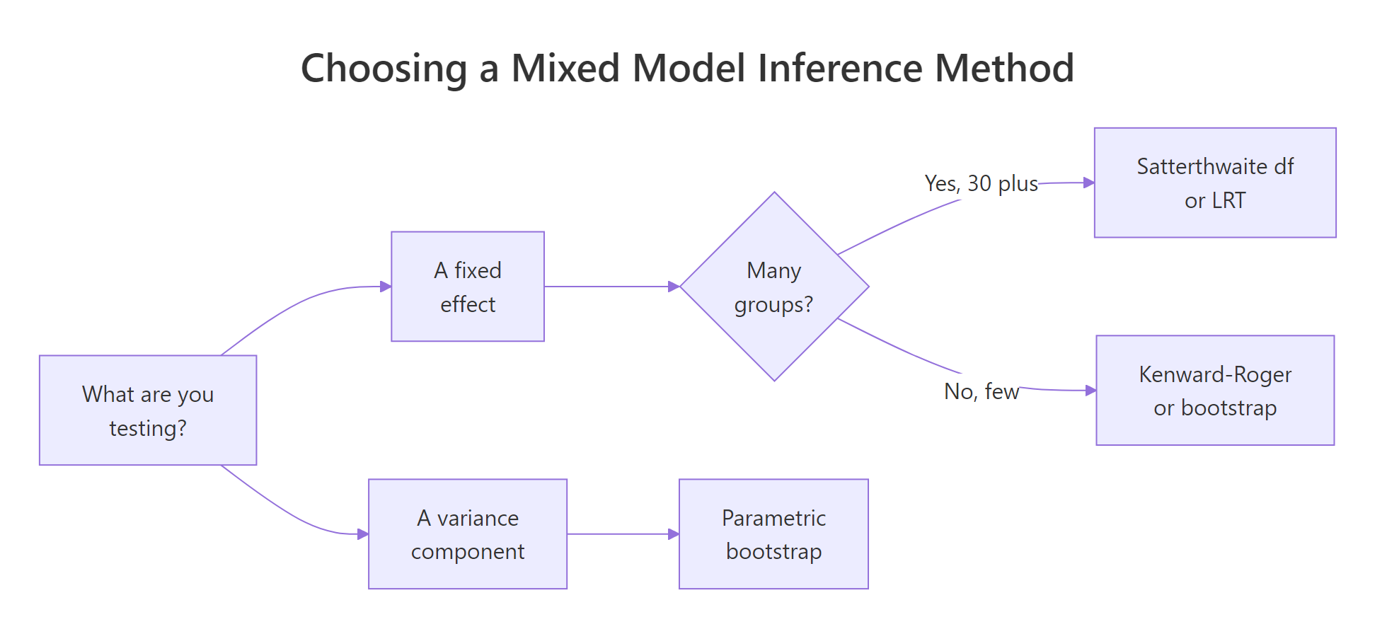
Figure 1: A quick guide to picking a mixed model inference method.
Here is the same advice as a table you can keep next to your keyboard.
| Method | Best for | Runs in R with | Watch out for |
|---|---|---|---|
| t-as-z (Wald) | A fast gut-check | base lme4 | Too optimistic with few groups |
| Likelihood ratio test | Fixed effects, decent sample | base lme4 (anova) |
Refit with REML = FALSE first |
| Satterthwaite df | Per-coefficient p-values | lmerTest |
Linear (Gaussian) models only |
| Kenward-Roger df | Small samples, safest df method | lmerTest + pbkrtest |
Slower on big models |
| Parametric bootstrap | Variance components, awkward cases | lme4, pbkrtest |
Needs many simulations, time |
For an everyday linear mixed model, Kenward-Roger or Satterthwaite p-values plus a profile confidence interval will serve you well. Switch to the bootstrap when you are testing a variance component or when your groups are few and you want a method that leans on no distributional shortcut.
Try it: Encode the "how many groups" part of the rule as a helper function.
Click to reveal solution
Explanation: The cutoff of 30 groups is a common rule of thumb, not a hard law; with borderline group counts, prefer the safer small-sample method.
Complete Example: comparing every method on one slope
Let's bring the fixed-effect methods together for the Days slope in one table, so you can see them side by side. This reuses the objects built earlier in the tutorial (fm, p_approx, null_ml, fm_ml, and boot_slope), assembling their answers into a single data frame.
Every method points to the same conclusion: the Days slope is about 10.5 ms per day, clearly different from zero, with a confidence interval roughly from 7 to 14. The p-values differ in scale (the t-as-z one is the smallest, because it is the most optimistic), but they all sit far below any sensible threshold. When your methods agree like this, you can report the result with confidence. When they disagree, the disagreement itself is telling you the approximations are strained, and the bootstrap is your tie-breaker.
Practice Exercises
These combine several ideas from the tutorial. Try each before opening the solution. The exercises use distinct variable names so they will not overwrite the objects built above.
Exercise 1: Is the random slope earning its place?
So far we let each subject have their own slope with (Days | Subject). Test whether that added flexibility is justified against a simpler model where subjects share one common slope but keep their own intercept, (1 | Subject). Refit both by maximum likelihood and compare them with a likelihood ratio test.
Click to reveal solution
Explanation: The tiny p-value says the per-subject slopes matter, so the random slope stays. One caution: because this test is about variance components sitting on a boundary, the reported p-value is actually a little conservative (too large), so a borderline result here would deserve a bootstrap test rather than the naive chi-squared.
Exercise 2: Does the model's standard error match the bootstrap?
The Std. Error in the summary table is itself an approximation. Check it by bootstrapping the Days slope 200 times and comparing the standard deviation of the bootstrap estimates to the model's reported standard error.
Click to reveal solution
Explanation: The bootstrap standard error (1.406) is close to the model's (1.546), which is reassuring. The bootstrap value is slightly smaller because it does not assume the errors are perfectly normal; a large gap between the two would warn you the model-based standard error is unreliable.
Exercise 3: A bootstrap prediction interval
Point predictions deserve uncertainty too. Estimate the mean reaction time on Day 5 for a typical subject (using only the fixed effects), and put a 95% bootstrap interval around it.
Click to reveal solution
Explanation: The same bootMer engine bootstraps any function of the model, including a prediction. A typical subject is predicted to react in about 304 ms on Day 5, plausibly between 286 and 321 ms.
Frequently Asked Questions
Why does lmer give p-values once I load lmerTest but not before?
Loading lmerTest replaces the plain lmer with a version that estimates the denominator degrees of freedom (using Satterthwaite by default) and adds the p-value column. The underlying model fit is identical; only the summary method changes. Base lme4 leaves the column out because it will not commit to a single degrees-of-freedom rule.
Should I fit with REML or maximum likelihood?
Use REML (the default) for your final estimates and confidence intervals, because it gives less biased variance components. Switch to REML = FALSE only when you run a likelihood ratio test that compares different fixed effects, since REML likelihoods are not comparable across those models. The Satterthwaite and Kenward-Roger methods work fine on REML fits.
Which p-value should I actually report?
For an ordinary linear mixed model, report the Kenward-Roger or Satterthwaite p-value, since simulation studies show they control false positives best. Add a profile or bootstrap confidence interval so readers see the effect size and its uncertainty, not just a yes/no verdict.
My model prints "boundary (singular) fit". Is my inference still valid?
A singular fit means a variance or correlation is estimated at its boundary (often zero), which makes p-values and standard errors for the random effects unreliable. Simplify the random-effects structure (for example, drop a correlation or a random slope), then rerun the inference on the simpler model. See common lme4 convergence warnings for the full playbook.
Do these methods work for logistic or Poisson mixed models?
The likelihood ratio test and the parametric bootstrap work for generalized linear mixed models (GLMMs) fit with glmer. The Satterthwaite and Kenward-Roger degrees-of-freedom methods do not, because they are built for the Gaussian case. For a GLMM, lean on the bootstrap or the LRT.
Summary
Mixed models withhold p-values because the denominator degrees of freedom are genuinely uncertain, and this tutorial gave you five honest ways to supply the missing inference.
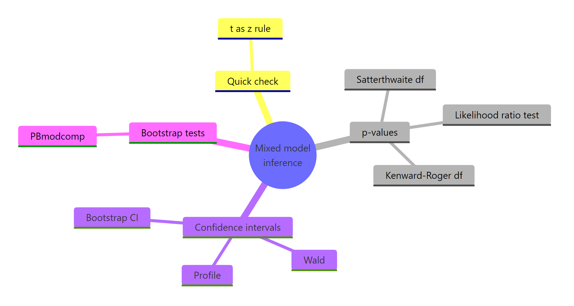
Figure 2: The mixed model inference toolbox at a glance.
| Takeaway | What to remember |
|---|---|
| No p-value column is intentional | The exact degrees of freedom for lmer are unknown |
| t-as-z is a shortcut, not a report | Fine when far from the boundary, risky near it |
| Likelihood ratio test needs ML | Refit with REML = FALSE, then anova() |
| Satterthwaite and Kenward-Roger | Best default p-values for linear mixed models, via lmerTest |
| Confidence intervals beat p-values | Wald is fast, profile is more accurate, bootstrap assumes least |
| Bootstrap is the tie-breaker | Simulate, refit, collect; use many simulations and a seed |
If your methods agree, report the result with confidence. If they disagree, the parametric bootstrap is your tie-breaker.
References
- Bates, D., et al. lme4 reference: getting p-values for fitted models. Link
- lme4 reference: bootMer, model-based parametric bootstrap for mixed models. Link
- lme4 reference: confint.merMod, Wald, profile, and boot confidence intervals. Link
- Kuznetsova, A., Brockhoff, P. B., Christensen, R. H. B. lmerTest Package: Tests in Linear Mixed Effects Models. Journal of Statistical Software (2017). Link
- Halekoh, U., Hojsgaard, S. A Kenward-Roger Approximation and Parametric Bootstrap Methods for Tests in Linear Mixed Models (pbkrtest). Journal of Statistical Software (2014). Link
- Luke, S. G. Evaluating significance in linear mixed-effects models in R. Behavior Research Methods (2017). Link
- Bolker, B. GLMM FAQ: testing hypotheses and computing p-values. Link
Continue Learning
- Random Intercepts and Slopes with lme4 - how to build the mixed model whose coefficients we test here.
- Likelihood Ratio Tests and Pivotal Methods - the theory behind the LRT, generalized to any nested-model comparison.
- The Bootstrap in R - the resampling idea from the ground up, before the mixed-model twist.