Measurement Reliability in R: Alpha, ICC, Agreement
Measurement reliability is the degree to which a measurement reflects a real, stable signal instead of random noise. In R you quantify it three ways: Cronbach's alpha for the internal consistency of a multi-item scale, the intraclass correlation (ICC) for agreement between raters on numeric scores, and Cohen's or Fleiss' kappa for agreement on categories.
What is measurement reliability, and why does it matter?
Every score you record is part real signal and part random noise. Reliability is simply the share that is signal. If two attempts to measure the same thing disagree wildly, the number is mostly noise, and any conclusion you build on it is unreliable too. The fastest way to feel this is to measure the same people twice and see how well the two attempts agree.
Let's build that demonstration. We invent 50 people with a fixed true ability, then measure each person twice with a precise instrument (small random error) and twice more with a sloppy one (large random error). Everything on this page uses base R unless a block says otherwise.
That correlation between two attempts at the same measurement is called test-retest reliability. The precise instrument reproduces itself almost perfectly (0.95), while the noisy one barely agrees with itself (0.39). Same 50 people, same true abilities: the only difference is how much random error each instrument adds.
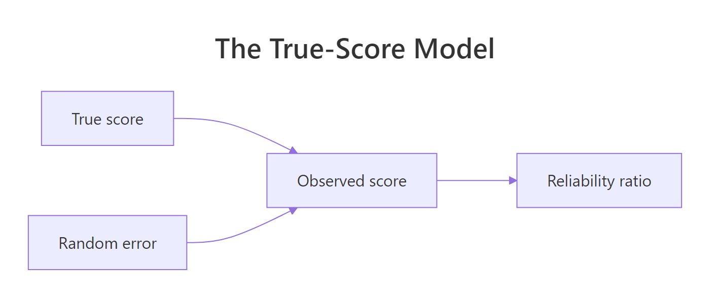
Figure 1: Every observed score splits into a true part and a random error part; reliability is the true part's share of the total.
The figure names the model behind that demo. An observed score equals a true score plus random error, and because the two are independent, the observed variance is the true variance plus the error variance. Reliability is the true variance divided by the observed variance. We simulated the data, so we actually know each person's true score and can compute that ratio directly.
The precise instrument is 93% signal, the noisy one only 52%. In real studies you never see the true score, so you cannot compute this ratio directly. The rest of this tutorial estimates that same signal share from data you can actually collect: several items answered by one person, or several raters judging the same subjects.
Try it: Build a third instrument that is noisier than the precise one but cleaner than the sloppy one by using rnorm(50, sd = 8) for its error, then report its test-retest correlation. Reuse true_score and remember to seed for reproducibility.
Click to reveal solution
Explanation: With error sd of 8, the test-retest correlation lands at 0.74, between the precise 0.95 and the noisy 0.39. More measurement error always lowers reliability.
How do you measure internal consistency with Cronbach's alpha?
Often you cannot measure someone twice, but you can ask several related questions at once. A questionnaire that measures job satisfaction might have seven items. If they all tap the same underlying idea, people who score high on one should tend to score high on the others. That "hang-togetherness" is internal consistency, and Cronbach's alpha is its most common summary.
R ships with a real survey dataset called attitude: 30 departments rated on seven aspects of workplace experience, each on a 0 to 100 scale. Let's look at the first three rows.
Each column is one item, each row is one department. Alpha asks a simple question: relative to the spread of the total score, how much of the variation is shared across items rather than private to each one. We can compute it straight from variances. Add up the variance of each item, compare that to the variance of the row totals, and scale by the number of items.
The seven items produce an alpha of 0.843. Here is the logic behind the arithmetic you just ran. If items were unrelated, the total variance would sit close to the sum of the item variances, the fraction inside the parentheses would fall near zero, and alpha would collapse toward zero. When items move together they reinforce each other, so the total variance grows well past the sum of the item variances. That shrinks the fraction and pushes alpha toward one.
$$\alpha = \frac{k}{k-1}\left(1 - \frac{\sum_{i=1}^{k} \sigma^2_{i}}{\sigma^2_{\text{total}}}\right)$$
Where:
- $k$ = the number of items (here 7)
- $\sigma^2_i$ = the variance of item $i$
- $\sigma^2_{\text{total}}$ = the variance of the summed total score
A close cousin, standardized alpha, ignores the raw variances and works only from the average correlation between items. It answers the same question on a cleaner footing when items use different scales.
The average item pair correlates at 0.427, and standardized alpha is 0.839, right next to the raw value. In practice you would reach for a package rather than retype these formulas every time.
install.packages(c("psych", "irr")), to reproduce the numbers.The alpha() function in the psych package returns the same coefficient plus a diagnostic you will want: what alpha would become if each item were dropped. Run this locally.
library(psych)
rel <- alpha(attitude)
round(rel$total[, c("raw_alpha", "std.alpha", "average_r")], 3)
#>  raw_alpha std.alpha average_r
#>      0.843     0.839     0.427
round(rel$alpha.drop[, "raw_alpha", drop = FALSE], 3)
#>            raw_alpha
#> rating         0.810
#> complaints     0.797
#> privileges     0.828
#> learning       0.803
#> raises         0.795
#> critical       0.864
#> advance        0.840
The headline numbers match your hand calculation exactly (0.843 and 0.839). The drop table is the useful part: alpha stays near 0.80 no matter which item you remove, except that dropping critical would push alpha up to 0.864. That item is the weak link, contributing little shared signal. How do you read the coefficient itself? Use this common guide.
| Cronbach's alpha | Interpretation |
|---|---|
| below 0.60 | Poor |
| 0.60 to 0.69 | Questionable |
| 0.70 to 0.79 | Acceptable |
| 0.80 to 0.89 | Good |
| 0.90 and above | Excellent |
Try it: Compute Cronbach's alpha for just three of the columns, complaints, learning, and raises, using the same by-hand recipe. Store the three-column data frame first.
Click to reveal solution
Explanation: Three strong items already reach 0.833, close to the full seven-item scale, which tells you those three carry most of the shared signal.
How do you measure rater agreement on numeric scores with the ICC?
Now change the setup. Instead of one person answering many items, several raters each score the same subjects on a numeric scale: judges scoring gymnasts, doctors rating scan severity, coders scoring essays. You want to know whether the subjects can be told apart reliably despite differences between raters. The intraclass correlation, or ICC, answers this by asking what share of the total variation comes from real differences between subjects rather than from rater disagreement or noise.
We use a small, published example from Shrout and Fleiss (1979): six targets each rated by four judges. Working with a known dataset lets you check the results against the literature.
Scan the rows and you can see the judges disagree a lot on the raw numbers (Judge2 is consistently harsh), yet they mostly rank the targets the same way. The ICC turns that impression into a number. The tool that separates the sources of variation is a two-way analysis of variance with target and judge as factors.
The ANOVA hands us three mean squares. MSR (11.24) measures how much the targets differ from each other, the real signal we hope dominates. MSC (32.49) measures how much the judges differ in overall strictness. MSE (1.02) is the leftover noise. The ICC formulas combine these three numbers, and the exact recipe depends on the question you are asking.
$$\text{ICC(3,1)} = \frac{MS_R - MS_E}{MS_R + (k-1)\,MS_E} \qquad \text{ICC(2,1)} = \frac{MS_R - MS_E}{MS_R + (k-1)\,MS_E + \frac{k}{n}(MS_C - MS_E)}$$
Where:
- $MS_R$ = the between-subjects mean square (real target differences)
- $MS_C$ = the between-raters mean square (judge strictness)
- $MS_E$ = the residual mean square (noise)
- $n$ = the number of subjects, $k$ = the number of raters
The two formulas differ in one place: the consistency version, ICC(3,1), ignores $MS_C$, while the absolute-agreement version, ICC(2,1), adds it as a penalty. Consistency forgives a judge who is harsh as long as they rank targets correctly; agreement demands that raters land on the same actual number. Let's compute both, plus the version for the average of all four judges.
Look at how far apart these are for the very same ratings. Judged on ranking alone, a single rater is fairly reliable (0.715). Demand that raters agree on the exact score and reliability drops to 0.29, because Judge2's harshness now counts against them. Average all four judges together and reliability jumps to 0.909, since pooling cancels individual quirks. The psych package computes all six standard forms at once, with confidence intervals. Run this locally.
res <- psych::ICC(ratings)$results
data.frame(form  = res$type,
           ICC   = round(res$ICC, 3),
           lower = round(res$`lower bound`, 3),
           upper = round(res$`upper bound`, 3))
#>    form   ICC  lower upper
#> 1  ICC1 0.166 -0.133 0.723
#> 2  ICC2 0.290  0.019 0.761
#> 3  ICC3 0.715  0.342 0.946
#> 4 ICC1k 0.443 -0.884 0.912
#> 5 ICC2k 0.620  0.071 0.927
#> 6 ICC3k 0.909  0.676 0.986
Your hand-computed values sit right in this table: ICC3 is 0.715, ICC2 is 0.290, ICC3k is 0.909. The six forms come from three yes-or-no choices, laid out below.
| psych label | Model | Type | Unit |
|---|---|---|---|
| ICC1 | One-way random | Absolute | Single rater |
| ICC2 | Two-way random | Agreement | Single rater |
| ICC3 | Two-way mixed | Consistency | Single rater |
| ICC1k | One-way random | Absolute | Average |
| ICC2k | Two-way random | Agreement | Average |
| ICC3k | Two-way mixed | Consistency | Average |
The irr package lets you request one specific form directly, which is handy when a journal asks for exactly the absolute-agreement single-rater value. Run this locally.
library(irr)
icc(ratings, model = "twoway", type = "agreement", unit = "single")
#>  Single Score Intraclass Correlation
#>    Model: twoway
#>    Type : agreement
#>    Subjects = 6
#>      Raters = 4
#>    ICC(A,1) = 0.29
#>    F(5,15) = 11 , p = 0.000135
#>  95%-Confidence Interval for ICC Population Values:
#>   0.019 < ICC < 0.761
That confirms the by-hand agreement value of 0.29 once more. To interpret any ICC, the widely used Koo and Li (2016) guideline is a good default.
| ICC | Reliability |
|---|---|
| below 0.50 | Poor |
| 0.50 to 0.75 | Moderate |
| 0.75 to 0.90 | Good |
| above 0.90 | Excellent |
Try it: You have MSR, MSC, MSE, and n in memory from the ANOVA. Compute the absolute-agreement ICC for the average of the four judges, ICC(2,k), whose formula is (MSR - MSE) / (MSR + (MSC - MSE) / n).
Click to reveal solution
Explanation: Averaging the four judges lifts absolute agreement from 0.29 for a single rater to 0.62 for the panel mean, matching ICC2k in the psych table. More raters, averaged, cancel individual bias.
How do you measure agreement on categories with Cohen's kappa?
Sometimes raters do not give numbers at all: they assign categories. Two examiners grade essays as Fail, Pass, Merit, or Distinction; two doctors label a scan as benign or malignant. The obvious measure is the percentage of cases the raters label the same way, but that number overstates agreement, because raters agree by pure luck a fair amount of the time. Cohen's kappa fixes this by subtracting the agreement expected from chance.
Here are two examiners grading the same 20 essays. We store the grades as ordered factors and cross-tabulate them into a confusion table.
The diagonal counts the essays both examiners graded identically. Everything off the diagonal is a disagreement. Adding up the diagonal and dividing by 20 gives the raw agreement.
They agree on 15 of 20 essays, or 75%. That sounds decent, but part of it is luck. If both examiners hand out Pass often, they will land on Pass together sometimes even without reading the essays. Kappa asks how much of the 75% is real skill beyond that chance floor.
$$\kappa = \frac{p_o - p_e}{1 - p_e}$$
Where:
- $p_o$ = the observed proportion of agreement (0.75 here)
- $p_e$ = the proportion of agreement expected by chance, from the row and column totals
To get the chance floor, multiply each grade's row share by its column share and add across grades. That is the agreement you would expect if each examiner threw grades independently while keeping their overall habits.
Chance alone would produce about 27% agreement, so the raw 75% is a lot better than luck. Kappa rescales the gap into 0.66, meaning the examiners captured about two thirds of the possible agreement above chance.
The irr package computes kappa directly, and it can also weight disagreements. For ordered grades, a Fail-versus-Distinction mix-up is worse than a Merit-versus-Distinction slip, and squared weights penalize far-apart disagreements more heavily. Run this locally.
grades <- data.frame(examiner_A, examiner_B)
kappa2(grades, weight = "unweighted")
#>  Cohen's Kappa for 2 Raters (Weights: unweighted)
#>  Subjects = 20
#>    Raters = 2
#>     Kappa = 0.66
kappa2(grades, weight = "squared")
#>  Cohen's Kappa for 2 Raters (Weights: squared)
#>     Kappa = 0.718
The unweighted kappa reproduces your 0.66. The squared-weight version rises to 0.718, because the examiners' disagreements were all near misses between neighbouring grades rather than wild swings, and weighting rewards that. When you have three or more raters, Cohen's kappa no longer applies, but Fleiss' kappa extends the same chance-corrected idea to a whole panel. Run this locally.
set.seed(9)
ticket_ratings <- matrix(c(
  1, 1, 1, 2, 2, 2, 3, 3, 3, 1, 1, 2, 2, 2, 3,
  3, 3, 3, 1, 1, 1, 2, 3, 2, 1, 1, 1, 2, 2, 2,
  3, 3, 3, 1, 2, 1, 2, 2, 2, 3, 3, 3, 1, 1, 1),
  ncol = 3, byrow = TRUE)
kappam.fleiss(ticket_ratings)
#>  Fleiss' Kappa for m Raters
#>  Subjects = 15
#>    Raters = 3
#>     Kappa = 0.733
Three coders labelling 15 support tickets into three categories reach a Fleiss' kappa of 0.733. To judge any kappa, the Landis and Koch (1977) scale is the classic reference.
| Kappa | Agreement |
|---|---|
| below 0.00 | Poor |
| 0.00 to 0.20 | Slight |
| 0.21 to 0.40 | Fair |
| 0.41 to 0.60 | Moderate |
| 0.61 to 0.80 | Substantial |
| 0.81 to 1.00 | Almost perfect |
Try it: Two coders labelled 10 emails as Spam or Ham. Build the confusion table with table(), then compute both raw agreement and Cohen's kappa by hand. The two label vectors are provided.
Click to reveal solution
Explanation: The coders agree on 8 of 10 emails (0.8 raw), but after removing the chance floor the kappa is 0.6, moderate agreement. The correction matters even for a tidy binary task.
How do you choose the right reliability measure?
The three coefficients are not competitors; each fits a different shape of data. The deciding question is what your ratings look like, as the figure and table below lay out.
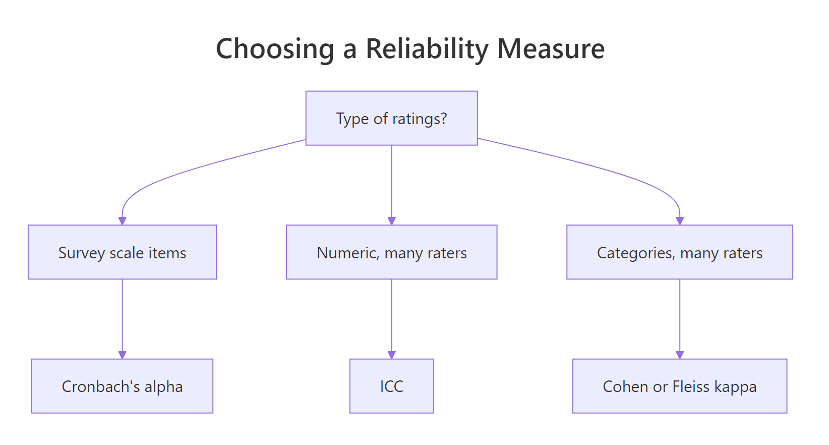
Figure 2: Pick the reliability measure from the kind of ratings you have.
| You have | You want to know | Use |
|---|---|---|
| Many items, one construct | Internal consistency | Cronbach's alpha |
| Numeric scores, several raters | Rater reliability | Intraclass correlation |
| Category labels, two raters | Agreement beyond chance | Cohen's kappa |
| Category labels, three or more raters | Agreement beyond chance | Fleiss' kappa |
Complete Example: an end-to-end reliability check
Let's put ICC and kappa on the same dataset to see how the lens changes the answer. Three interviewers score 10 job candidates on a 0 to 10 scale. First we generate and view the panel.
Treating the scores as numbers, we ask how reliable the panel is when we average all three interviewers, using the absolute-agreement ICC for the mean of the raters.
As a numeric panel, reliability is excellent at 0.926. Now suppose the company only cares about a yes-or-no call: recommend a candidate whose score is 6 or higher. We collapse two interviewers' scores into that decision and measure agreement with Cohen's kappa.
Here is the lesson. The same interviewers whose numeric scores were 0.926 reliable drop to a kappa of 0.6, only moderate, once you flatten the scores into a yes-or-no verdict. Dichotomizing throws away the fine gradations that made the panel look strong. When a numeric scale exists, keep it and report the ICC rather than reducing everything to a coarse label.
Practice Exercises
These combine several ideas from the tutorial. Each solution runs on its own, so try it before you reveal the answer.
Exercise 1: Find the weakest item in a scale
Build a five-item scale from the columns complaints, privileges, learning, raises, and advance. Compute Cronbach's alpha for the full scale, then compute alpha with each item removed in turn. Which single item, if dropped, raises alpha the most, and what does that tell you about that item?
Click to reveal solution
Explanation: Dropping advance lifts alpha to 0.837, just above the full-scale 0.835. Every other removal lowers alpha. That makes advance the weakest contributor: it adds items to the scale without adding much shared signal.
Exercise 2: Compute an ICC from scratch
Three raters scored six subjects, giving the matrix below. Using only base R, run a two-way ANOVA and compute the single-rater consistency ICC, ICC(3,1), from the mean squares. Its formula is (MSR - MSE) / (MSR + (k - 1) * MSE).
Click to reveal solution
Explanation: These raters barely disagree, so almost all the variation reflects real subject differences, giving an excellent single-rater ICC of 0.91.
Exercise 3: The base-rate trap
Two radiologists screened 100 scans for a rare disease. Their agreement is summarized in the 2-by-2 table below: both radiologists called 80 scans negative and 5 positive, and they disagreed on 10 scans split evenly in each direction. Compute the raw agreement and Cohen's kappa, then explain why they tell such different stories.
Click to reveal solution
Explanation: Raw agreement is a comfortable 0.85, but kappa is only 0.318, merely fair. Because the disease is rare, both radiologists say "negative" most of the time and agree by default, so the chance floor is high and little genuine skill is left to credit. This is exactly why kappa, not raw percentage, is the honest measure for skewed categories.
Summary
Measurement reliability is one idea, the signal's share of the total variation, measured three ways depending on the shape of your data. The mindmap below is your recap, and the table pins each family to its R tools.
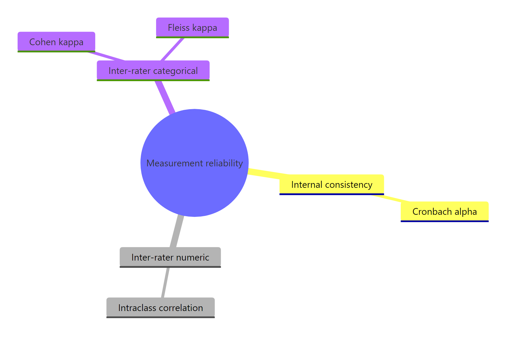
Figure 3: The three families of reliability and their coefficients.
| Family | Question it answers | By hand in R | Package function | Rule of thumb |
|---|---|---|---|---|
| Internal consistency | Do these items measure one thing? | item and total variances | psych::alpha() | alpha 0.80 or higher is good |
| Rater reliability (numeric) | Do raters score subjects alike? | two-way ANOVA mean squares | psych::ICC(), irr::icc() | ICC 0.75 or higher is good |
| Rater agreement (categorical) | Do raters pick the same category? | confusion table, chance correction | irr::kappa2(), irr::kappam.fleiss() | kappa 0.61 or higher is substantial |
Key takeaways to carry forward:
- Reliability is a proportion of variance, so it always sits between 0 and 1, and higher means less noise.
- Cronbach's alpha rewards items that move together, but a high alpha does not guarantee the scale is one-dimensional.
- The ICC has several forms; always state the model, and whether it describes a single rater or an average.
- Kappa beats raw percent agreement because it removes the agreement raters would reach by chance.
- Collapsing numeric ratings into categories can turn an excellent ICC into a merely moderate kappa, so keep the finer scale when you can.
FAQ
What counts as a good Cronbach's alpha?
A common rule treats 0.70 as acceptable, 0.80 as good, and 0.90 as excellent for research scales. Values above 0.95 can actually signal redundant items that ask the same question twice, so higher is not always better.
What is the difference between Cronbach's alpha and the ICC?
Alpha summarizes how well several items on one questionnaire hang together to measure a single construct. The ICC summarizes how well several raters agree when they each score the same subjects. They answer different questions, though both express reliability as a share of variance.
Why use Cohen's kappa instead of raw percent agreement?
Raw percent agreement counts every match, including the ones raters would hit by chance. Kappa subtracts that expected chance agreement, so it is not inflated when one category is very common. The base-rate exercise above shows raw agreement of 0.85 shrinking to a kappa of 0.318.
Which ICC form should I report?
Pick the form that matches your design and use. Choose two-way if the same raters score every subject, absolute agreement if the exact score matters (not just the ranking), and single-rater if one rater will score future cases alone. Report the choice alongside the value.
Does a high reliability score mean my measurement is accurate?
No. Reliability is about consistency, not correctness. A scale that reads five pounds heavy gives the same wrong number every time, so it is perfectly reliable yet completely inaccurate. Reliability is necessary for a good measure but not sufficient: to show that a measure captures the right thing, you also need validity evidence, such as a factor analysis that the items load on the intended construct or a comparison against an external standard.
Can a reliability coefficient be negative?
Yes. Cronbach's alpha and the ICC can dip below zero when items or raters disagree more than chance would predict, which usually points to a reverse-coded item or a genuine measurement problem rather than a low-but-valid reliability.
References
- Cronbach, L. J. (1951). Coefficient alpha and the internal structure of tests. Psychometrika. Link
- Shrout, P. E., & Fleiss, J. L. (1979). Intraclass correlations: uses in assessing rater reliability. Psychological Bulletin. Link
- Koo, T. K., & Li, M. Y. (2016). A guideline of selecting and reporting intraclass correlation coefficients. Journal of Chiropractic Medicine. Link
- Landis, J. R., & Koch, G. G. (1977). The measurement of observer agreement for categorical data. Biometrics. Link
- McHugh, M. L. (2012). Interrater reliability: the kappa statistic. Biochemia Medica. Link
- Revelle, W. psych: Procedures for Psychological, Psychometric, and Personality Research. CRAN. Link
- Gamer, M., et al. irr: Various Coefficients of Interrater Reliability and Agreement. CRAN. Link
- R Core Team. An Introduction to R. Link
Continue Learning
- Factor Analysis in R: confirm that your questionnaire items really measure one underlying construct before you trust their alpha.
- Correlation Analysis in R: the pairwise correlation is the building block underneath both alpha and the ICC.
- Statistical Tests in R: round out your toolkit for comparing groups and validating measures.