Random Intercepts and Slopes with lme4 in R
Random intercepts and slopes let a single model give every group in your data its own baseline and its own trend, while still sharing what all the groups have in common. This guide builds that idea from scratch on one small dataset, shows you how to fit the model with the lme4 package, and walks through every line of the output so you can read it with confidence. It uses base R plus lme4, and the examples run right here in your browser.
Why do repeated measurements need random intercepts and slopes?
Most real datasets are not a flat list of independent rows. They come in groups: several test scores per student, many visits per patient, repeated readings per sensor. When you measure the same subject more than once, those measurements are related to each other, and pretending they are independent leads you astray. Random intercepts and slopes are the tool that respects that grouping.
We will work with sleepstudy, a dataset that ships with lme4. It records the reaction time (in milliseconds) of 18 people across 10 days of restricted sleep. Each person was measured once per day, so every person contributes 10 related rows. Let's load it and look.
Each row is one measurement. Reaction is the outcome we want to explain, Days is how long the person has been sleep-deprived, and Subject is the person's ID. The first four rows are all subject 308, which is the grouping we care about. Let's confirm the shape of the data.
So we have 18 subjects and 180 measurements, which works out to exactly 10 rows per person. That balanced, repeated structure is the classic setting for mixed models. The naive approach is to ignore Subject entirely and fit one straight line to all 180 points.
This says the average person starts around 251 ms and slows by about 10.5 ms per day. Treating all 180 rows as one pile is called complete pooling, because it pools every subject together and forgets who is who. The problem is that people are not the same, and forcing them onto one line hides that.
To see how different people really are, we can go to the opposite extreme and fit a separate line for each subject. The lmList() helper in lme4 does exactly that.
Look at the range. Subject 308 starts at 244 ms and degrades fast, at 21.8 ms per day, while subject 309 starts lower at 205 ms and barely changes, at 2.3 ms per day. The intercepts differ and the slopes differ. Fitting 18 completely separate lines is called no pooling, because each subject is estimated on its own with no help from the others.
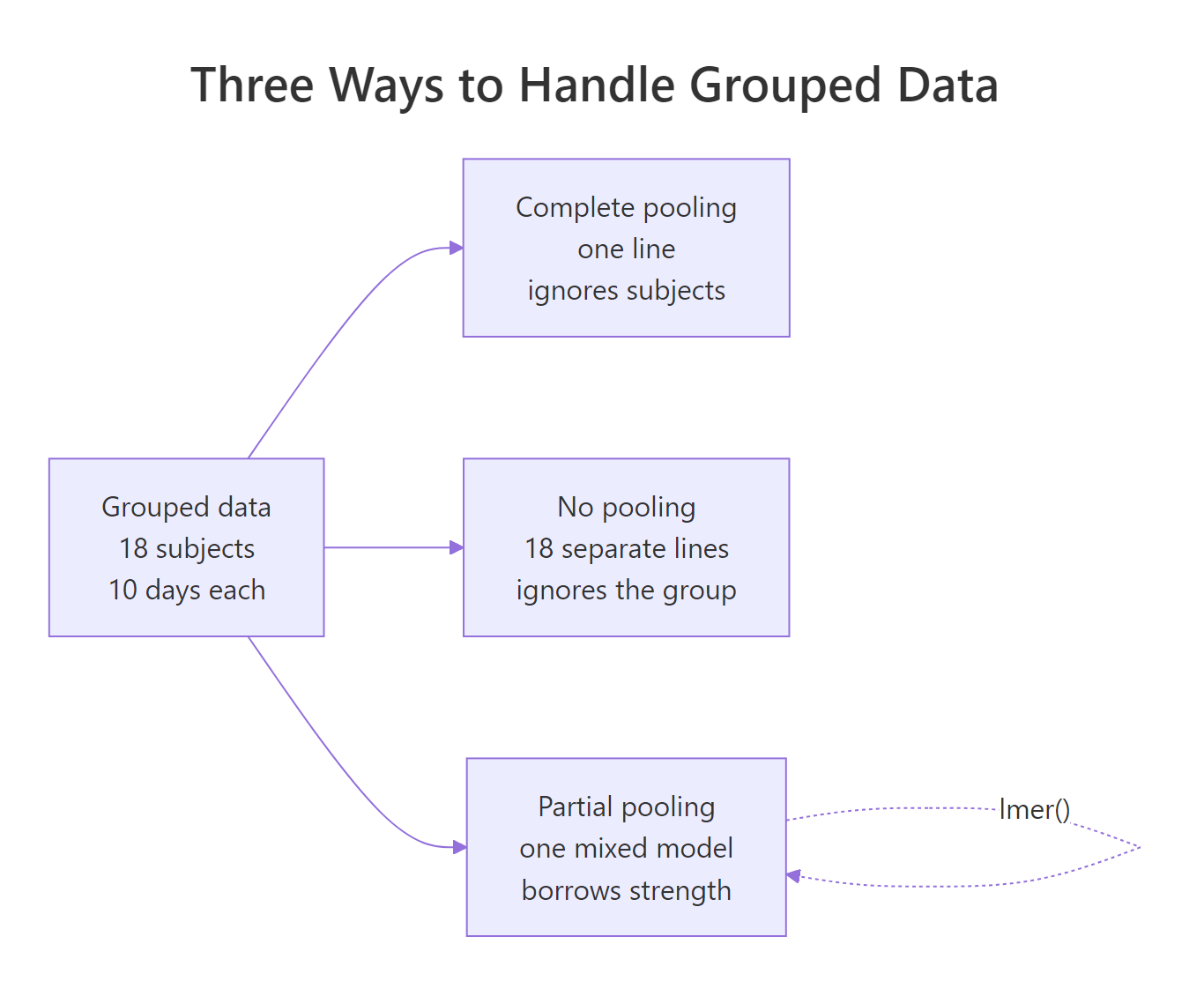
Figure 1: Three ways to handle grouped data; mixed models take the middle path.
Neither extreme is satisfying. Complete pooling throws away real differences between people, and no pooling throws away the fact that all 18 people are still humans doing the same task, so their lines should not be wildly independent. A mixed model takes the middle road, called partial pooling, and that is what random intercepts and slopes give you.
Try it: Pull out subject 309's own intercept and slope from the by_subject fit above. The row name you want is "309".
Click to reveal solution
Explanation: Subject 309 starts at about 205 ms and slows by only 2.3 ms per day. Indexing the lmList coefficients by the subject ID gives that subject's private OLS line.
What is a random intercept?
A random intercept is the simplest mixed model. It says every subject shares the same slope, but each one gets to shift the whole line up or down by their own amount. In plain terms, everyone degrades at the same rate, but some people are naturally faster or slower to begin with.
You fit it with lmer(), the mixed-model workhorse in lme4. The formula looks like an ordinary regression, Reaction ~ Days, plus a new piece in parentheses: (1 | Subject). Read that as "give each Subject its own intercept," because 1 is R's shorthand for the intercept.
This output has two halves, and telling them apart is the key skill. The bottom half, "Fixed effects," is the part that looks like ordinary regression. The average person starts at 251 ms and slows by 10.5 ms per day, which matches the pooled line from earlier. These are the effects that apply to everyone, so they are called fixed effects.
The top half, "Random effects," is the new part and it describes variation, not a single line. It reports two variances. The Subject (Intercept) standard deviation of 37.1 ms says that individual starting points scatter around the average intercept with a spread of about 37 ms. The Residual standard deviation of 31 ms is the day-to-day noise left over within a subject after the model accounts for the person.
Subject, not eighteen coefficients like the fixed effects in Read-lm-Output-in-R.You can still recover each subject's own line. The coef() function combines the shared fixed effects with each subject's personal deviation.
Notice the Days column is identical for every subject, at 10.47. That is the point of a random intercept model: the slope is shared, so the fitted lines are parallel, and only the intercept moves up or down. Subject 308 sits high at 292 ms and subject 309 sits low at 174 ms, but both slow at the same rate.
Try it: The ranef() function shows each subject's intercept deviation from the average, rather than the full intercept. Print the deviation for subject 330.
Click to reveal solution
Explanation: Subject 330 sits about 4.4 ms above the average intercept of 251.4 ms, which gives their personal intercept of about 255.8 ms, exactly what coef() reported.
How do you add a random slope?
A random intercept lets people start in different places, but our earlier per-subject fit showed that people also degrade at different rates. Subject 308 lost 21.8 ms per day while subject 309 lost only 2.3. To let the slope vary by subject, you add the predictor inside the parentheses: (Days | Subject). Read that as "give each Subject its own intercept and its own slope for Days."
The fixed effects barely moved: the average person still starts at 251 ms and slows by 10.5 ms per day. What changed is the random-effects block, which now has three lines instead of one. There is a spread for the intercept (24.7 ms), a brand new spread for the slope (5.9 ms per day), and a Corr column.
That slope spread is the heart of this model. It says subjects differ in their day-to-day degradation with a standard deviation of about 5.9 ms per day. Some people barely slow down while others slow much faster, and the model now measures how much that varies. The Corr value of 0.07 is the correlation between a subject's intercept and slope, telling you whether people who start slow also tend to degrade fast; here it is near zero, so the two are roughly unrelated.
The formula piece (Days | Subject) is doing several jobs at once, so it helps to break it apart.
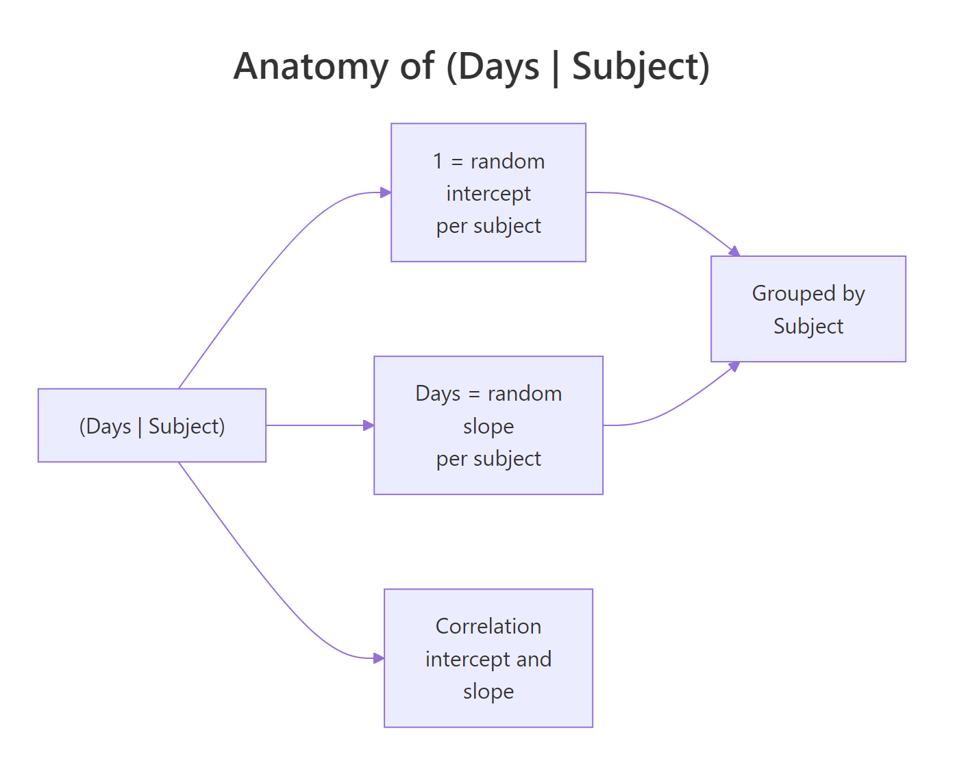
Figure 2: What each piece of (Days | Subject) tells lmer to estimate.
(Days | Subject) gives you a random slope for Days, a random intercept, and the correlation between them, all three at once. If you truly want a random slope with no random intercept, which is rare, you must write (0 + Days | Subject). Most of the time the default with the intercept is what you want.If you like seeing the model written out, here is what a random-intercept-and-slope model says for reaction time $y$ of subject $j$ on day $i$. If formulas are not your thing, skip past the equation to the next code block; the summary above already gives you the same information.
$$y_{ij} = (\beta_0 + b_{0j}) + (\beta_1 + b_{1j})\,x_{ij} + \epsilon_{ij}$$
Where:
- $\beta_0$ and $\beta_1$ = the fixed intercept and slope, shared by everyone
- $b_{0j}$ and $b_{1j}$ = subject $j$'s random shifts away from that shared intercept and slope
- $x_{ij}$ = the number of days of sleep deprivation
- $\epsilon_{ij}$ = the leftover within-subject noise
The random shifts $b_{0j}$ and $b_{1j}$ are the numbers summarized by those two standard deviations in the output. Now let's see each subject's full line, intercept and slope together.
Now the Days column varies. Subject 308 degrades at 19.7 ms per day while subject 309 barely moves at 1.8. Compare these to the separate-lines fit from the first section: 308 was 21.8 and 309 was 2.3. The mixed model gives numbers in the same neighborhood but nudged toward the group, which is the partial pooling we will unpack soon.
Try it: From the random-slope model, read subject 308's personal slope for Days out of coef(rs)$Subject. Round it to two decimals.
Click to reveal solution
Explanation: Subject 308 slows by about 19.7 ms per day, the steepest degradation among the people we have looked at, and well above the average of 10.5.
How do you read the random-effects table and get p-values?
The random-effects table is where beginners get stuck, so let's slow down on it. The cleanest way to see just those numbers is VarCorr(), which strips away the rest of the summary.
Each row is a source of variation. The intercept standard deviation of 24.7 ms is how much people differ in their starting reaction time. The Days standard deviation of 5.9 is how much they differ in their daily degradation. The residual of 25.6 ms is the noise left inside a subject once their personal line is accounted for. Reading these standard deviations, rather than the variances, keeps everything in the original millisecond units.
You may have noticed the summary printed no p-values for the fixed effects, only t value. That is deliberate. The author of lme4 argues that the exact degrees of freedom for these t statistics are not well defined for mixed models, so the package refuses to guess. You have two solid ways to get significance instead.
The first is a confidence interval, which many statisticians prefer anyway. The confint() function computes intervals for both the fixed effects and the variance components.
Read the bottom two rows first, since they are the fixed effects. The Days interval runs from 7.4 to 13.6 and does not include zero, so the average degradation is clearly real. The sd_Days|Subject interval runs from 3.8 to 8.8 and also stays well above zero, which is early evidence that subjects genuinely differ in their slopes, not just their intercepts.
If you want an actual p-value in the familiar format, the lmerTest package adds one by approximating the degrees of freedom. It is a standard CRAN package, but it is not part of the browser sandbox here, so run this block in a local R session.
library(lmerTest)
rs_p <- lmer(Reaction ~ Days + (Days | Subject), data = sleepstudy)
coef(summary(rs_p))
#>              Estimate Std. Error       df   t value     Pr(>|t|)
#> (Intercept) 251.40510   6.824597 16.99973 36.838090 1.171558e-17
#> Days         10.46729   1.545790 16.99998  6.771481 3.263824e-06
Now the Days effect carries a p-value of about 0.000003, comfortably significant. Notice the estimates and standard errors are identical to the plain lme4 fit; lmerTest only adds the degrees-of-freedom column and the resulting p-value, so nothing else about your model changes.
confint() output above gives you these for free.Try it: The residual standard deviation is the within-subject noise. Pull it straight out of the fitted model with sigma() and round it to two decimals.
Click to reveal solution
Explanation: After each subject's own line is fit, about 25.6 ms of day-to-day scatter remains. That matches the Residual row in the variance table.
Random intercepts vs random slopes: which do you need?
You now have two models: ri with only random intercepts, and rs with random intercepts and slopes. Adding a random slope costs extra parameters, so you should only keep it if it earns its place. The clean way to decide is a likelihood ratio test, which asks whether the bigger model fits significantly better than the smaller one. The anova() function runs it.
The test statistic is a chi-square of 42.1 on 2 degrees of freedom, with a p-value of 7e-10. That is tiny, so the random-slope model fits far better and you should keep it. In plain terms, subjects really do differ in how fast they degrade, not just in where they start, so forcing a shared slope would be wrong here.
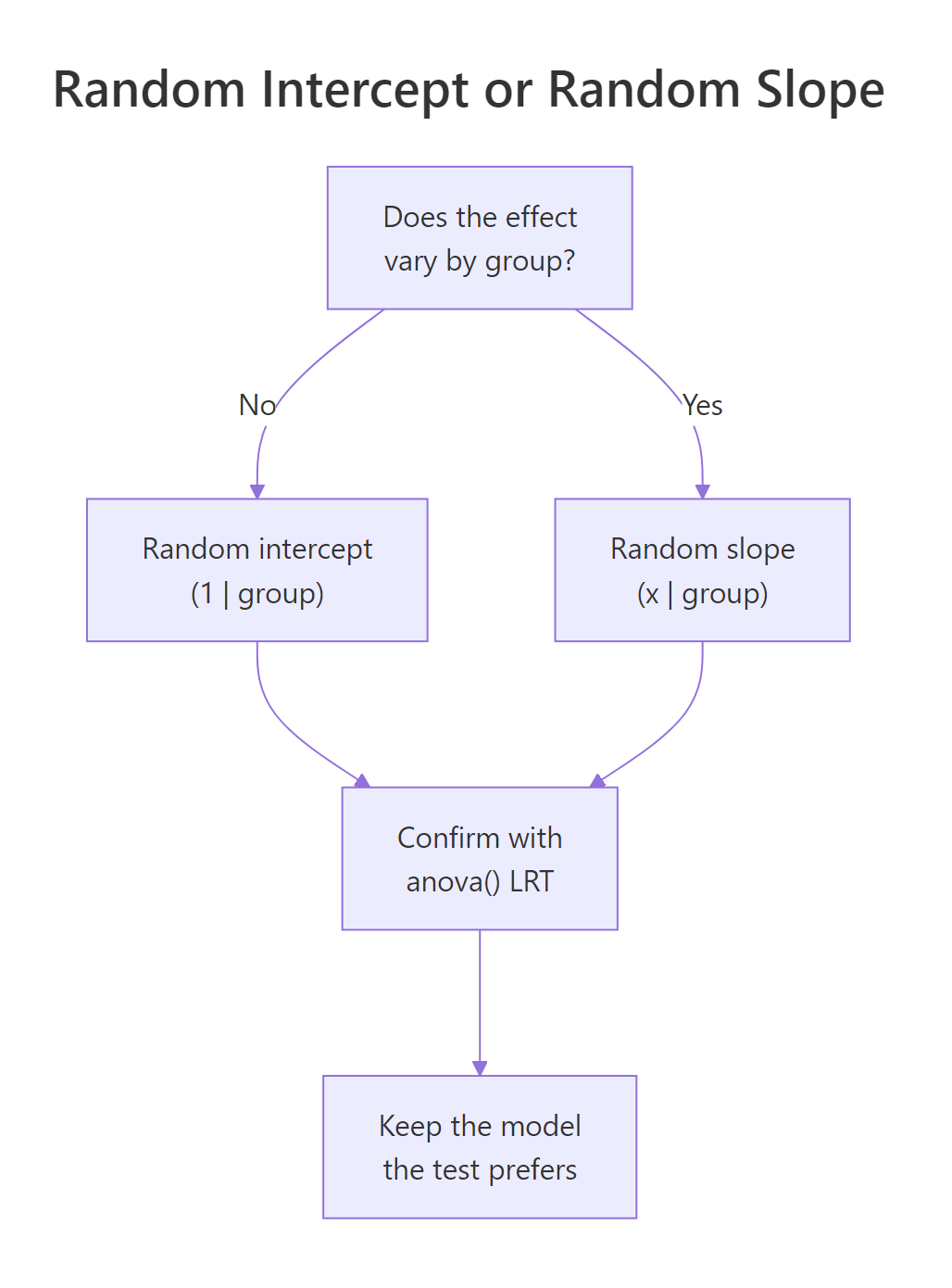
Figure 3: Deciding between a random intercept and a random slope.
AIC(ri, rs) directly gives 1794 and 1756. The gap is because lmer fits with REML by default for accurate variance estimates, but a likelihood ratio test needs plain maximum likelihood, so anova() quietly refits both models that way. Both routes agree the random-slope model wins.There is one subtlety worth knowing. This test checks whether a variance is zero, and zero sits on the edge of what a variance can be, since variances cannot go negative. That makes the standard p-value slightly conservative, meaning the true p-value is even smaller than reported. So when anova() says the random slope is significant, you can trust it comfortably.
Try it: Compare the two models by AIC instead, using AIC() directly on both fitted objects. Lower AIC is better.
Click to reveal solution
Explanation: The random-slope model scores 1756 against 1794 for the intercept-only model, an improvement of nearly 40 points, which strongly favors keeping the random slope.
How does partial pooling shrink each subject's line?
We keep saying a mixed model pulls each subject toward the group average. Now let's actually watch it happen by lining up the two extremes: the no-pooling slopes from the separate per-subject fits, and the partial-pooling slopes from the mixed model.
Every partial-pooling slope is closer to the group average than its no-pooling twin. The population slope is 10.5 ms per day, so watch the pull toward it. Subject 308's steep 21.8 is reined in to 19.7, subject 335's odd negative slope of -2.9 is pulled up to -0.3, and subject 331's shallow 5.3 is nudged up to 7.4. Extreme subjects move the most, and subjects near the average barely move.
The fixef() values are the center of gravity that every subject is pulled toward. This is why partial pooling is so useful: a subject with a noisy or extreme personal estimate gets stabilized by the group, while a subject with a clear signal keeps most of their own character.
Try it: Compute how far subject 335's slope was shrunk, the no-pooling slope minus the partial-pooling slope. Use the row names from the block above.
Click to reveal solution
Explanation: Subject 335's slope moved by 2.6 ms per day toward the group average. The negative sign shows the no-pooling estimate was below the pooled one, so shrinkage pulled it upward.
Practice Exercises
These exercises combine several ideas from the guide. Try each before opening the solution. They use their own variable names, prefixed with my_, so they will not disturb the models you fit above.
Exercise 1: Fit, compare, and find the steepest subject
Using sleepstudy, fit both a random-intercept model and a random-slope model, compare them with AIC, then find which subject has the steepest fitted slope in the random-slope model.
Click to reveal solution
Explanation: The random-slope model wins on AIC by nearly 40 points, and subject 308 has the steepest degradation of all 18 people, slowing fastest under sleep deprivation.
Exercise 2: A random slope on a different dataset
The built-in ChickWeight data tracks the weight of chicks over Time, grouped by Chick. Fit a random-intercept-and-slope model of weight on time, then print the fixed effects and the variance components. This proves the same recipe works on any grouped dataset.
Click to reveal solution
Explanation: The average chick starts near 29 grams and gains about 8.5 grams per unit time. The Time standard deviation of 3.76 shows chicks differ a lot in growth rate, and the strong negative correlation of -0.95 means chicks that start heavier tend to grow more slowly.
Exercise 3: Rebuild a subject's line by hand
Confirm you understand where each subject's line comes from. For subject 309 in the random-slope model rs, add the fixed effects to that subject's random deviations from ranef(), and check that the result matches coef(rs)$Subject.
Click to reveal solution
Explanation: Adding subject 309's random deviations to the fixed effects reproduces coef() exactly. This is the whole idea in one line: a subject's fitted line is the population line plus that subject's personal shifts.
Frequently Asked Questions
What is the difference between a fixed effect and a random effect?
A fixed effect is a single value estimated for the whole dataset, like the average slope of 10.5 ms per day that applies to everyone. A random effect is a set of group-specific deviations that are assumed to follow a bell curve, summarized by a variance rather than by one coefficient per group. Use a fixed effect when you care about the specific levels, and a random effect when the levels are a sample from a larger population, like these 18 subjects standing in for people in general.
When should I use (1 | group) versus (x | group)?
Use (1 | group) when groups differ only in their baseline level, so parallel lines are enough. Use (x | group), which is short for (1 + x | group), when the effect of x itself varies by group, so the lines need different slopes. A likelihood ratio test with anova() tells you whether the extra random slope is worth its cost, as it was in this guide.
Why does lme4 not print p-values?
The exact degrees of freedom for the t statistics in a mixed model are not well defined, so lme4 deliberately reports the t value without a p-value rather than print a number it cannot justify. To get a p-value, load the lmerTest package, which approximates the degrees of freedom, or report a confidence interval from confint() instead. Many analysts prefer the confidence interval because it shows the effect size and its uncertainty together.
What does a singular fit or boundary warning mean?
A "boundary (singular) fit" warning means the model pushed a variance to zero or a correlation to plus or minus one, usually because the random-effects structure is too complex for the data to support. The fix is to simplify: drop the correlation with (Days || Subject), or remove the random slope and keep only (1 | Subject). The full random-slope model on sleepstudy fits cleanly, so you will not see the warning here, but you will meet it on smaller datasets.
How many groups do I need for a random effect?
A rough rule of thumb is at least 5 to 10 groups, and ideally more than 20, before a variance component is estimated reliably. With very few groups, the spread of the random effect is hard to pin down, and you are often better off treating the grouping variable as a fixed effect with dummy variables. The 18 subjects in sleepstudy sit comfortably in the workable range. Everything in this guide also runs unchanged in a local RStudio session; install lme4 once with install.packages("lme4").
Summary
Random intercepts and slopes let one model give every group its own line while sharing an overall trend, which is exactly what repeated-measurement data needs. You fit them with lmer(), choose the random structure with a likelihood ratio test, and read variation from the random-effects table rather than from a coefficient per group.
| Formula piece | What it does | When to use it | |
|---|---|---|---|
Days |
Fixed effect: one shared slope for everyone | Always, for the average trend | |
| `(1 \ | Subject)` | Random intercept: each group shifts up or down | Groups differ in baseline only |
| `(Days \ | Subject)` | Random intercept and slope, correlated | Groups differ in the effect too |
| `(0 + Days \ | Subject)` | Random slope with no random intercept | Rare, only when baseline is truly shared |
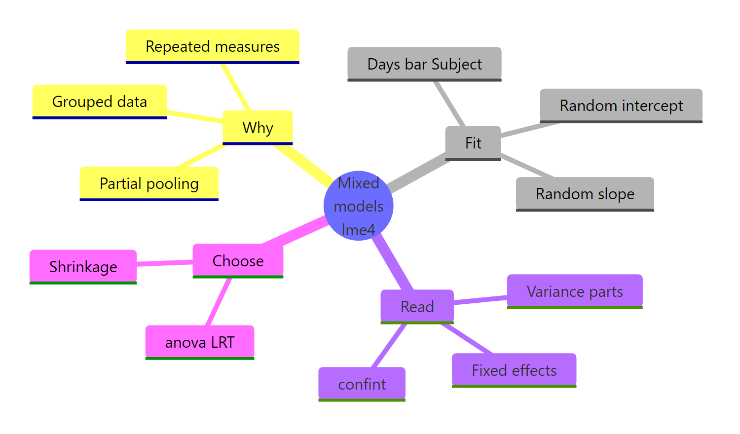
Figure 4: The whole workflow at a glance.
The biggest ideas to carry with you: fixed effects describe the average and random effects describe the spread, the bar term (x | group) quietly adds a random intercept too, and partial pooling shrinks extreme groups toward the average so your estimates stay sensible.
References
- Bates, D., Mächler, M., Bolker, B., & Walker, S. (2015). Fitting Linear Mixed-Effects Models Using lme4. Journal of Statistical Software, 67(1). Link - the canonical paper behind
lme4, with the theory and syntax forlmer(). - lme4 package vignette: Fitting Linear Mixed-Effects Models Using lme4. Link - the official walkthrough, including the
sleepstudyexample used here. - lme4 on CRAN. Link - the package home, with the reference manual and installation notes.
- Clark, M. Mixed Models with R: More Random Effects. Link - a clear, extended treatment of random slopes and variance components.
- Mahr, T. Plotting Partial Pooling in Mixed-Effects Models. Link - the best visual explanation of shrinkage, built on
sleepstudy. - DeBruine, L., & Barr, D. J. Learning Statistical Models Through Simulation in R. Link - a simulation-first introduction to mixed models.
- Bolker, B. GLMM FAQ. Link - practical answers on p-values and singular fits, plus how many groups you really need.
Continue Learning
- How to Read lm() Output in R - the fixed-effects half of a mixed model is just ordinary regression, and this covers how to read it.
- Linear Regression in R - the straight-line model that random intercepts and slopes extend to grouped data.
- GLM Diagnostics in R - once your model is fit, these checks confirm its assumptions hold.