Offsets and Exposure in Poisson Models in R
An offset is a fixed term you add to a Poisson model so it predicts a rate (events per unit of exposure) instead of a raw count. It is the natural logarithm of the exposure, and its coefficient is locked at 1 rather than estimated. This guide builds the idea from a two-clinic example up to a full car-insurance model, all in base R with glm(), and shows how to read the results as rate ratios and turn them into predictions.
Why do raw counts mislead when exposure differs?
A count is only a fair comparison when every group had the same chance to accumulate events. The moment one group is observed longer, or contains more people, or covers more ground, it will log more events for no interesting reason. Exposure is that background amount of opportunity, and ignoring it is one of the most common mistakes in count modeling. Let's see it happen with two hospital clinics tracking infections over one year.
Look at the raw counts first: Clinic B recorded 42 infections against Clinic A's 24, so B looks worse. Now look at the last column. Clinic B saw 600 patients while A saw only 200, and once we express each as infections per 100 patients, B's rate is 7 and A's rate is 12. The clinic with more infections actually has the lower infection rate.
The fix was to divide each count by its exposure, here the number of patients, to get a rate everyone can be compared on. That single division is the whole intuition behind offsets. The rest of this guide is about doing the same thing inside a model, so we can add predictors and get uncertainty estimates on the rates.
Try it: Health reports usually quote infections per 1000 patients, not per 100. Change the multiplier so ex_per_1000 holds the rate per 1000 patients for each clinic.
Click to reveal solution
Explanation: Swapping 100 for 1000 rescales the rate. Clinic A sits at 120 infections per 1000 patients and Clinic B at 70. The ranking is unchanged because the denominator is the same for both; only the units moved.
What is an offset in a Poisson model?
A Poisson regression models a count using a log link, which means it predicts the logarithm of the expected count from a straight-line combination of your predictors. If you have not met it yet, think of it as the count-data cousin of ordinary linear regression, fitted with glm(y ~ x, family = poisson). On its own it models counts, but we just saw that counts are the wrong target when exposure varies. We want it to model the rate.
Here is the small piece of algebra that gets us there. If formulas are not your thing, skip to the code below: the three lines just say to drop log(exposure) into the model with its slope pinned to 1. Writing $\mu_i$ for the expected count of observation $i$, a plain Poisson model is:
$$\log(\mu_i) = \beta_0 + \beta_1 x_i$$
We actually care about the rate, which is the expected count divided by the exposure $t_i$. So put the rate inside the log instead:
$$\log\!\left(\frac{\mu_i}{t_i}\right) = \beta_0 + \beta_1 x_i$$
Using the rule that $\log(a/b) = \log(a) - \log(b)$, move the exposure to the other side:
$$\log(\mu_i) = \beta_0 + \beta_1 x_i + \log(t_i)$$
Where:
- $\mu_i$ = the expected event count for observation $i$
- $t_i$ = the exposure for observation $i$ (patient-days, person-years, population, area)
- $x_i$ = a predictor value
- $\beta_0, \beta_1$ = the coefficients R estimates
That extra $\log(t_i)$ on the end is the offset. It looks like a predictor, but notice it has no coefficient of its own to estimate. Its multiplier is fixed at 1, because doubling the exposure should exactly double the expected count. Exposure shows up in many fields under different names, so it helps to see the pattern.
| Field | Event (the count) | Exposure (the denominator) |
|---|---|---|
| Epidemiology | new infections | person-years at risk |
| Insurance | claims filed | policies or policy-years |
| Manufacturing | defects found | units produced |
| Ecology | animals seen | area surveyed |
| Traffic safety | crashes | miles driven |
To make the rest of this concrete, let's simulate a realistic dataset. Imagine 300 hospital wards, each observed for a different number of patient-days, where half used a new hygiene protocol that truly cuts the infection rate to 60% of the standard rate.
Each row is one ward with its infection count, its exposure, and its protocol. Because every ward ran for a different number of patient-days, the raw infections column is not comparable across rows. Let's pool the wards by protocol and compute the rate the same way we did for the clinics.
Standard wards ran up 1419 infections across 48655 patient-days, a rate of 29.2 per 1000 patient-days. The new-protocol wards recorded 991 infections over 54220 patient-days, a rate of 18.3. The ratio of the two rates, 18.3 divided by 29.2, is about 0.63, which is close to the true value of 0.60 we built into the simulation. An offset model will recover exactly this rate ratio while also giving us a confidence interval and room for more predictors.
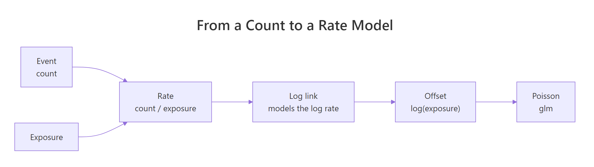
Figure 1: How a raw count becomes a rate model through the log link and an offset.
Try it: Using the totals table above, compute the rate ratio for the new protocol by dividing its rate by the standard rate. You should land near 0.63.
Click to reveal solution
Explanation: Dividing the two pooled rates gives 0.627, meaning the new protocol's infection rate is roughly 63% of the standard rate. This hand calculation is exactly what the model will estimate in a moment, only the model adds a confidence interval.
How do you fit an offset with glm() in R?
You fit an offset with the same glm() you would use for any Poisson model, and you name the exposure inside an offset() wrapper in the formula. The exposure goes in on the log scale, so you write offset(log(patient_days)), matching the algebra above. Let's fit the ward model and read the summary.
Read the coefficients on the log scale for now, we will convert them to rates in the next section. The intercept of -3.535 is the log baseline rate for the reference group, standard wards. The protocolnew coefficient of -0.467 is the change in log rate for switching to the new protocol, and its tiny p-value says that change is very unlikely to be chance. Everything here is the log of a rate per patient-day, because the offset accounts for the exposure.
R gives you a second way to supply the offset: a dedicated offset = argument, separate from the formula. It fits the identical model, so use whichever reads more clearly to you.
The coefficients match m to every decimal, confirming the two syntaxes are interchangeable. The formula version keeps the exposure visible next to your predictors, while the argument version keeps the formula short. Neither is more correct.
offset(patient_days) instead of offset(log(patient_days)) silently fits a different and wrong model, so double-check the log is there.Try it: Refit the ward model, but pass the exposure through the offset = argument instead of inside the formula. Confirm the coefficients still match m.
Click to reveal solution
Explanation: Adding offset = log(patient_days) produces the same intercept and slope as the formula-based m. The starter code left the offset out, which would have fitted a count model that ignores how long each ward was watched.
Why fix the exposure coefficient at 1 instead of estimating it?
It is fair to ask why we bolt the exposure in with a fixed coefficient of 1 rather than letting the model estimate its effect like any other predictor. The answer is that fixing it at 1 is what makes the model a rate model. A coefficient of 1 on log(exposure) says that doubling the exposure doubles the expected count exactly, which is the definition of a constant rate. Let's test that assumption by freeing the coefficient and seeing where it lands.
Now log(patient_days) is an ordinary predictor with its own estimated coefficient, and that coefficient came out at 0.983, very close to 1. When the data really do behave like a rate, the freed coefficient hovers around 1, which is a reassuring check that the offset assumption fits. Let's confirm that 1 is a plausible value with a confidence interval.
The 95% interval runs from 0.90 to 1.07, and it comfortably contains 1. That means the data give us no reason to reject the fixed-at-1 offset, so the simpler rate model is justified. If instead the interval sat well away from 1, it would be a signal that events do not scale proportionally with exposure, and you might keep exposure as a free predictor or rethink the exposure measure.
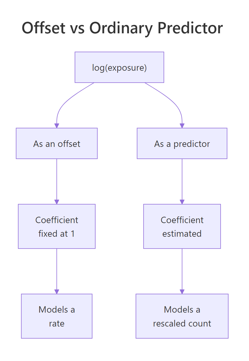
Figure 2: The same log(exposure) term means two different models depending on whether its coefficient is fixed or estimated.
Try it: Pull just the log(patient_days) coefficient out of m_cov and round it to two decimals, so you can quote how close the freed exposure effect is to 1.
Click to reveal solution
Explanation: Indexing the coefficient vector by name isolates the exposure effect, which rounds to 0.98. That is close enough to 1 that fixing it as an offset costs almost nothing and buys a clean rate interpretation.
How do you read the coefficients as rate ratios?
Log-scale coefficients are hard to feel, so the standard move is to exponentiate them. Taking exp() of a coefficient turns it into a rate ratio, often called an incidence rate ratio: the factor by which the rate multiplies when that predictor changes by one unit. Doing the same to the confidence limits gives you an interval on the rate ratio. Let's convert the whole ward model at once.
Start with the intercept: its rate ratio of 0.0292 is the baseline rate itself, about 29 infections per 1000 patient-days for standard wards, which matches the pooled number we computed by hand earlier. The protocolnew rate ratio of 0.627 is the headline result. Switching to the new protocol multiplies the infection rate by 0.627, a reduction of about 37%. Because the confidence interval, 0.58 to 0.68, sits entirely below 1, we can say the drop is statistically clear, not noise.
Try it: Convert the protocolnew coefficient into a percentage change in the rate. A rate ratio of 0.627 should come out near a 37% reduction.
Click to reveal solution
Explanation: Subtracting 1 from the rate ratio and multiplying by 100 converts it to a percentage change. The value of -37.3 means the new protocol is associated with a 37.3% lower infection rate, the plain-language version of the rate ratio 0.627.
How do you predict rates and counts from the model?
A fitted offset model can answer two different questions: how many events to expect, and at what rate. The key is that predict(..., type = "response") returns an expected count and automatically includes whatever exposure you supply in the new data. So to predict a count, give the real exposure; to predict a rate, fix the exposure at a chosen unit. Let's predict counts first, for a standard and a new ward each watched for 500 patient-days.
Over 500 patient-days, the model expects about 14.6 infections in a standard ward and 9.1 in a new-protocol ward. Those are counts, and they carry the exposure of 500 baked in. To get a rate instead, we fix the exposure at a fixed reference amount, say 1000 patient-days, so the offset becomes the same constant for every row and the prediction reads as a rate per 1000.
Setting the exposure to 1000 turns the predicted count into a rate per 1000 patient-days: 29.2 for standard wards and 18.3 for new. These match the pooled rates from the very first ward table, confirming the model recovered the empirical rates exactly, now with the machinery to add predictors and intervals.
Try it: Predict the expected number of infections for a single new-protocol ward observed for 250 patient-days.
Click to reveal solution
Explanation: With 250 patient-days of exposure, the model expects about 4.6 infections in a new-protocol ward. That is half the 9.1 it predicted for 500 patient-days, exactly as a constant rate demands when you halve the exposure.
Complete Example: Modeling Car Insurance Claim Rates
Let's put the whole workflow together on real data. The Insurance dataset in the MASS package records, for groups of British car-insurance policyholders in 1973, how many claims each group filed and how many policyholders it contained. The number of policyholders is the exposure, because a group with more drivers will file more claims even if each driver is no riskier. We coerce the two ordered factors to plain factors so the coefficients read as simple group comparisons.
Each row is a group of policyholders described by district, engine size (Group), and driver age band, with Holders as the exposure and Claims as the count. We model the claim rate with district, engine size, and age as predictors, and log(Holders) as the offset.
The signs are already easy to read. Bigger engines carry positive coefficients that grow with engine size, so larger cars claim at a higher rate. Older age bands carry negative coefficients that grow more negative with age, so older drivers claim at a lower rate. To make those readable, exponentiate every coefficient into a rate ratio.
Now each number is a multiplier on the claim rate relative to its reference group. Drivers over 35 have a rate ratio of 0.585, meaning they claim at about 59% of the rate of the under-25 reference band, a 41% lower rate. The largest engines carry a rate ratio of 1.757, so they claim at roughly 76% above the smallest-engine reference. District 4 stands out among districts at 1.264. Finally, let's turn the model into a business forecast: the expected number of claims from a group of 3000 young drivers in District 1 with the smallest engines.
The model expects about 485 claims from those 3000 policyholders, which is a rate of roughly 0.16 claims per holder, the baseline rate for this highest-risk profile. Because we passed the real Holders count of 3000, this comes back as a count you could plug straight into a reserving calculation. Swap in a different exposure and you would get the forecast for a differently sized book of business.
Practice Exercises
These pull together fitting, rate ratios, prediction, and the offset-versus-covariate idea. Each uses distinct variable names so it will not overwrite the tutorial objects.
Exercise 1: Report a rate ratio with its interval
Using the wards data, fit a Poisson model of infections on protocol with offset(log(patient_days)), then report the new-protocol rate ratio together with its 95% confidence interval. Save the fit as my_fit. You should recover a rate ratio near 0.63.
Click to reveal solution
Explanation: Exponentiating the coefficient and its Wald interval gives a rate ratio of 0.627 with a 95% CI of 0.58 to 0.68. Because the interval is entirely below 1, the new protocol's rate reduction is statistically clear.
Exercise 2: Rank age bands and forecast claims
Using the Insurance model, report the rate ratios for the three older age bands relative to the under-25 reference, then predict the expected claims for 5000 policyholders over 35 in District 1 with the smallest engines. Save the fit as my_ins.
Click to reveal solution
Explanation: The claim rate falls steadily with age, from 0.826 for 25-29 down to 0.585 for over-35, each relative to the youngest band. The forecast for 5000 older, small-engine, District 1 drivers is about 473 claims, lower per holder than the young-driver profile despite the larger group.
Exercise 3: Show what ignoring exposure does
This is the payoff exercise. Fit two models of Claims on Age alone: one with no offset, and one with offset(log(Holders)). Compare the age rate ratios. The no-offset model will give nonsense because older bands simply contain more policyholders.
Click to reveal solution
Explanation: Without the offset, the over-35 band looks like it claims 9 times as often as the youngest, purely because it holds far more policyholders. Add offset(log(Holders)) and the estimate flips to a rate ratio of 0.608, a 39% lower rate. Exposure was the confounder all along, and the offset removed it.
Frequently Asked Questions
Is an offset the same as a weight in glm()?
No. An offset shifts the linear predictor by a known amount and is the right tool for exposure. A weight in the weights = argument changes how much each row influences the fit, which answers a different question. For rate modeling of counts, you want the offset.
Does the exposure always have to be logged?
Yes, when you use the standard log link for Poisson regression. The model works on the log scale, so the exposure must enter as log(exposure) to line up with the algebra. Passing the raw exposure fits a different, incorrect model.
Can I use an offset with negative binomial models too?
Yes. Overdispersed counts are often fitted with MASS::glm.nb(), which accepts the very same offset(log(exposure)) term in the formula. The offset idea carries over unchanged; only the error distribution differs.
What if some rows have zero exposure?
You cannot log a zero, so log(0) is undefined and those rows break the model. A row with zero exposure also had no opportunity for an event, so it carries no rate information. Drop such rows before fitting.
Why not just model the rate directly as the response?
Because a rate is a ratio of a count to an exposure, and modeling it as a plain number throws away the count nature that makes the Poisson distribution appropriate. The offset lets you keep the integer count as the response while still targeting the rate, which is both more correct and better behaved for small counts.
Summary
Offsets are the bridge between counts and rates. When exposure varies across your rows, you fold log(exposure) into a Poisson model as an offset, a term whose coefficient is fixed at 1, and the model then estimates rates instead of raw counts. The table below is your quick reference.
| Task | Code |
|---|---|
| Fit with offset in the formula | glm(y ~ x + offset(log(E)), family = poisson) |
| Fit with the offset argument | glm(y ~ x, offset = log(E), family = poisson) |
| Rate ratio for a predictor | exp(coef(m)) |
| Rate ratio with interval | exp(cbind(coef(m), confint.default(m))) |
| Predict an expected count | predict(m, newdata, type = "response") with the real exposure |
| Predict a rate | same call with exposure fixed at a common value |
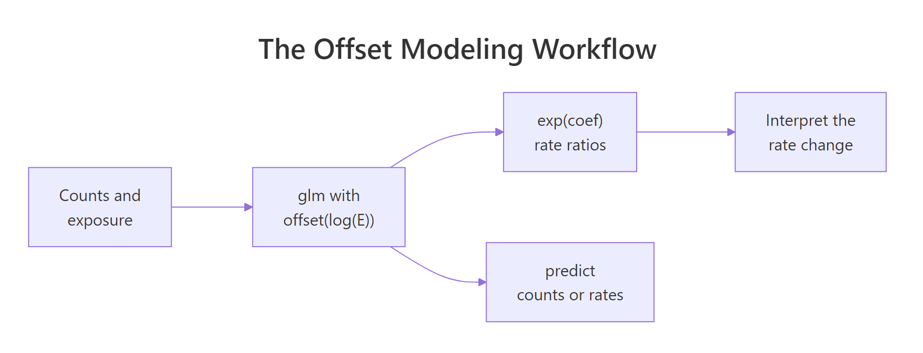
Figure 3: The offset modeling workflow from raw counts to interpreted rate ratios.
The core habits to keep: log the exposure, exponentiate coefficients into rate ratios you can explain in plain words, and decide between a count answer and a rate answer by what exposure you feed to predict(). Get those right and Poisson models with offsets become one of the most practical tools in applied statistics.
References
- R Core Team. glm() function documentation. Link
- R Core Team. family() and link functions in R. Link
- Venables, W. N. and Ripley, B. D. Insurance dataset reference (MASS package). Link
- Venables, W. N. and Ripley, B. D. Modern Applied Statistics with S, 4th Edition. Link
- MASS package on CRAN. Link
- UCLA Office of Advanced Research Computing. Poisson Regression in R. Link
- Musa, K. I. Poisson Regression, Data Analysis in Medicine and Health using R. Link
- R Core Team. An Introduction to R. Link
Continue Learning
- Poisson Regression in R: the foundation this guide builds on, covering the log link and count modeling from the start.
- Poisson and Negative Binomial Regression: what to do when counts are overdispersed and a plain Poisson model underestimates uncertainty.
- How to Read Logistic Regression Output in R: the same coefficient-reading skills applied to the other workhorse GLM.