Paired Designs in R: Before-After and Matched Pairs
A paired design measures the same subject twice (before and after) or matches subjects into pairs, so each pair acts as its own control. Analyzing the within-pair differences strips out person-to-person noise, which gives a far more sensitive test than comparing two separate groups. This tutorial builds the whole workflow in base R, from the first test to effect size and sample-size planning.
What is a paired design, and when do you use one?
Suppose the same 10 patients each tried two different sleep drugs, and you recorded how many extra hours they slept on each. The question is simple: did one drug help more than the other? Because every patient took both drugs, the two columns of numbers are linked patient by patient. That link is what makes the design "paired", and R has a one-argument switch to use it. The sleep dataset ships with R, so you can run the test right now.
Read the result from the bottom up. The average difference is 1.58, so drug 2 added about 1.58 more hours of sleep per patient than drug 1. The p-value of 0.0028 is well below 0.05, so that difference is unlikely to be chance. The 95% confidence interval runs from 0.70 to 2.46 hours and never touches zero, which tells the same story: the drugs really do differ.
Now let us look at the data that produced that answer, so the structure is clear. Each patient appears in two rows, one per drug.
There are 20 rows but only 10 patients, because each patient contributes two measurements. A before-after design looks exactly like this: the same person, measured at two time points. A matched pairs design is its close cousin, where you pair up two different people who are alike (twins, or two customers with similar histories) and give each a different treatment. Both designs share one idea: compare within the pair, not across the whole sample.
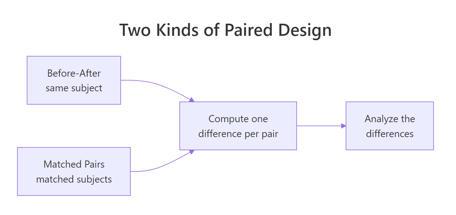
Figure 1: The two paired designs both reduce to one difference per pair.
Try it: Compute the mean extra sleep for each drug group so you can see the two averages behind that 1.58 difference.
Click to reveal solution
Explanation: tapply() splits extra by group and applies mean() to each piece. The gap of 2.33 minus 0.75 equals 1.58, the mean difference the paired test reported.
Why does pairing beat two independent samples?
It is tempting to think of the two drugs as two separate groups and reach for the ordinary two-sample t-test. Let us do exactly that on the very same data and see what happens. This is the test you get if you forget the paired = TRUE switch.
The group means are identical to before (0.75 and 2.33), yet the p-value jumped to 0.079, above the usual 0.05 line. The unpaired test would tell you there is no significant difference. Same numbers, opposite conclusion. The unpaired test threw away the pairing, and with it, the test's power.
Why does that happen? The unpaired test measures each drug's spread across all patients, and patients vary a lot in how much they sleep. The paired test instead looks at each patient's change, and those changes are much tighter. The numbers below make the gap visible.
The spread of the raw readings is about 2.02 hours, but the spread of the within-patient changes is only 1.23. The paired test divides by that smaller number, so the same 1.58 difference looks much bigger relative to the noise. The correlation of 0.80 is the reason: patients who slept a lot on drug 1 also slept a lot on drug 2, so subtracting removes that shared tendency.
Try it: The paired test uses the standard error of the differences. Compute it as the standard deviation of diffs divided by the square root of the number of pairs.
Click to reveal solution
Explanation: Dividing the mean difference (1.58) by this standard error (0.389) gives 4.06, exactly the t-statistic the paired test reported.
How do you run a paired t-test step by step?
Here is the idea that makes the paired t-test easy to understand: it is nothing more than a one-sample t-test run on the column of differences. You already built that column above as diffs. Testing whether its mean is zero is the same as testing whether the two conditions differ.
The t-statistic (4.0621), degrees of freedom (9), and p-value (0.002833) are identical to the paired test from the first section. That is not a coincidence, it is the definition. A paired t-test computes the differences for you and runs a one-sample test on them.
If you like seeing the machinery, the t-statistic is the mean difference divided by its standard error. If formulas are not your thing, skip the next block; the code above is all you need.
$$t = \frac{\bar{d}}{s_d / \sqrt{n}}$$
Where:
- $\bar{d}$ is the mean of the paired differences
- $s_d$ is the standard deviation of the differences
- $n$ is the number of pairs
Let us plug the pieces in by hand and confirm they reproduce the statistic.
The hand computation gives t = 4.0621 with 9 degrees of freedom, matching R's built-in output. This is why the test needs so little: just one column of differences plus its mean and spread.
Try it: Pull the 95% confidence interval for the mean difference out of a one-sample t-test on diffs.
Click to reveal solution
Explanation: Every t.test() result is a list, and $conf.int grabs the interval directly, which is handy when you want to report it without printing the full test.
How do you get before-after data into the right shape?
Real datasets rarely arrive pre-split into two neat vectors. The most common shape is wide: one row per subject, with a before column and an after column. Let us build a small weight-loss study in that shape and run the test straight from the columns.
Subjects lost 2.875 kg on average (p = 0.0012), and the interval from 1.58 to 4.17 kg stays positive. The other common shape is long: one row per measurement, with a column saying whether it is a before or after value. Many plotting and modeling tools prefer long format, so it helps to reshape with pivot_longer().
Each subject now spans two rows, tagged before or after. To run the paired test from long data, pull the two groups back out as vectors and keep them in subject order so the pairs line up.
Same t-statistic, same p-value. The shape of the data did not change the answer, only how you fed it to the test. A picture makes the pairing obvious: draw one line per subject connecting their before and after value.
Almost every line slopes downward, which is the visual signature of a real effect in a paired design. If the lines crossed randomly, the paired test would find little.
Try it: Using weight_long, compute the mean weight at each time point with group_by() and summarise().
Click to reveal solution
Explanation: The two means differ by 2.875 kg, matching the paired test. group_by() plus summarise() is the tidyverse way to collapse each group to a single number.
How do you check assumptions, and what if they fail?
The paired t-test makes one real assumption, and it is easy to get wrong. The assumption is that the differences are roughly normally distributed. Not the before values, not the after values, only their difference. With eight differences that is a lot to ask of a formal test, but shapiro.test() gives a quick read.
The Shapiro-Wilk p-value is 0.20, above 0.05, so there is no evidence the differences depart from normality. A picture helps confirm it. Plot the distribution of the differences and check that it is not wildly skewed or spiked.
When the differences are clearly non-normal, for example when an outlier dominates or the sample is small and skewed, switch to the Wilcoxon signed-rank test. It ranks the size of the differences instead of using their raw values, so a single extreme point has far less influence on the result. The decision comes down to one question, shown below.
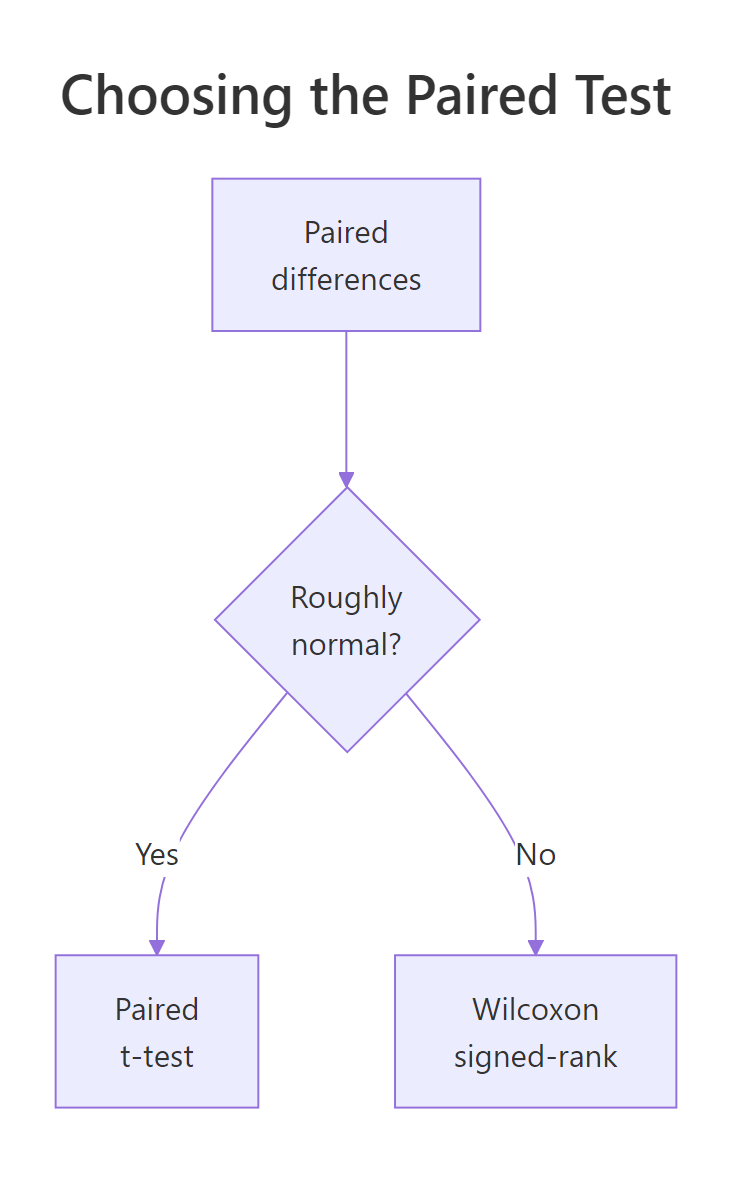
Figure 2: Normal differences point to the paired t-test; skewed ones to Wilcoxon.
Here is the Wilcoxon test on a small, skewed reaction-time sample where two values are far larger than the rest.
The test reports V = 36 and p = 0.0078, so reaction times dropped after the change even though the sample was skewed. The Wilcoxon test gives you a p-value without trusting the normality assumption.
Try it: Run a Shapiro-Wilk test on the sleep diffs you built earlier to see whether the paired t-test was justified there.
Click to reveal solution
Explanation: Here the p-value (0.033) dips just below 0.05, a mild warning that the differences are not perfectly normal. With only 10 pairs the paired t-test is fairly robust, but a cautious analyst would also report the Wilcoxon result as a cross-check.
How big is the effect, and how many pairs do you need?
A p-value tells you whether an effect exists, not how large it is. With enough pairs, even a trivial difference becomes "significant". So always report an effect size next to the p-value. For paired data the standard measure is Cohen's $d_z$: the mean difference divided by the standard deviation of the differences.
$$d_z = \frac{\bar{d}}{s_d}$$
It answers "how many standard deviations of change is the average change?" Rough guideposts are 0.2 (small), 0.5 (medium), and 0.8 (large).
A $d_z$ of 1.29 is very large: the typical patient's change is more than one standard deviation of change. That is why the effect was significant even with just 10 patients. The flip side of that question is planning: if you were designing a new study, how many pairs would you need to detect this effect reliably? Base R's power.t.test() answers it.
The answer is n = 6.9, which you round up to 7 pairs. Because the effect is so strong, a tiny study can detect it. For a type = "paired" calculation, remember that sd is the standard deviation of the differences, not of the raw scores, exactly as the note at the bottom of the output reminds you.
Try it: Compute Cohen's $d_z$ for the weight-loss study using weight_diffs.
Click to reveal solution
Explanation: A $d_z$ of 1.85 is a huge effect, which fits the near-parallel downward lines you saw in the slope plot.
Complete Example: a full before-after analysis
Let us tie every step together on a fresh study. Imagine 15 people ran a reaction-time task before and after a training program, with times recorded in milliseconds. We will simulate the data with a fixed seed so your run matches exactly, then walk the full pipeline: build the data, check the assumption, run the test, then report the effect.
The data is in wide format, one row per person. Next, form the differences, check that they are normal, then run the paired test.
The Shapiro-Wilk p-value of 0.65 says the differences are comfortably normal, so the paired t-test is appropriate. The test finds a mean drop of 25.8 ms with a tiny p-value, and the confidence interval from 17.6 to 34.0 ms stays well away from zero. Finally, package the result the way you would in a report, with the effect size included.
That single line is exactly what belongs in a results section: the size of the effect, its confidence interval, the test statistic with degrees of freedom, the p-value, and the standardized effect size. Any reader can judge both significance and practical importance from it.
Practice Exercises
These combine several steps from the tutorial. Try each before opening the solution. The starter blocks define the data for you, so you only write the analysis.
Exercise 1: Reshape and run a paired test
A blood-pressure study measured six patients before and after a drug. Reshape the wide table to long format, then run a paired t-test comparing before against after.
Click to reveal solution
Explanation: The drug lowered blood pressure by about 6.8 mmHg on average (p = 0.0007). Reshaping did not change the test, it just organized the data; the two vectors still had to be extracted in patient order.
Exercise 2: Pick the right test
An income-change sample has one enormous outlier. Compute the differences, test them for normality, then run the appropriate test: a paired t-test if the differences look normal, otherwise the Wilcoxon signed-rank test.
Click to reveal solution
Explanation: The Shapiro-Wilk p-value is far below 0.05, so the differences are not normal and the paired t-test is unsafe. The Wilcoxon test reports p = 0.27, so once you stop letting the outlier dominate, the change is not significant.
Exercise 3: Effect size and required sample size
Using the reaction-time train_diff from the Complete Example, compute Cohen's $d_z$, then use power.t.test() to find how many pairs would give 90% power at the observed effect.
Click to reveal solution
Explanation: The effect is large ($d_z$ = 1.74), so only about 6 pairs (rounding 5.7 up) are needed for 90% power. Strong effects need small samples; weak effects need large ones.
Frequently Asked Questions
When should I use a paired test instead of a two-sample test?
Use a paired test whenever each observation in one condition has a natural partner in the other: the same subject measured twice, or two subjects matched on key traits. If the two groups are unrelated people with no pairing, use the ordinary two-sample t-test.
Is a paired t-test really the same as a one-sample t-test on the differences?
Yes, exactly. The paired test computes each pair's difference and runs a one-sample t-test checking whether the mean difference is zero. You saw both routes give identical t, df, and p-values above.
What is the key assumption of the paired t-test?
That the paired differences are approximately normally distributed. The raw before and after values do not need to be normal, only their difference. Check it with shapiro.test() on the differences and a quick histogram.
What if my differences are not normal?
Use the Wilcoxon signed-rank test, wilcox.test(x, y, paired = TRUE). It ranks the differences rather than using their raw magnitudes, so outliers and skew have far less influence. With large samples the paired t-test also becomes robust to non-normality.
Is the analysis different for before-after versus matched pairs?
No. Both designs produce one difference per pair, and the math from that point on is identical. The difference is only in how the pairing arises: repeated measurement of one subject, or matching of two subjects.
How do I report a paired t-test?
Report the mean difference with its 95% confidence interval, the t-statistic with degrees of freedom, the p-value, and an effect size such as Cohen's $d_z$. The one-line report in the Complete Example shows the standard format.
Summary
Paired designs are one of the simplest ways to get a more sensitive test: by making each pair its own control, they remove the person-to-person noise that weakens two-sample comparisons. The table below captures the workflow.
| Step | What you do | R tool |
|---|---|---|
| Recognize the design | Same subject twice, or matched subjects | before-after / matched pairs |
| Shape the data | Wide (two columns) or long (one per row) | pivot_longer() |
| Visualize | One line per pair | ggplot() slope plot |
| Check the assumption | Differences roughly normal | shapiro.test() on differences |
| Run the test | Paired t-test, or Wilcoxon if skewed | t.test(..., paired = TRUE), wilcox.test(..., paired = TRUE) |
| Report the effect | Effect size and required sample size | Cohen's $d_z$, power.t.test() |
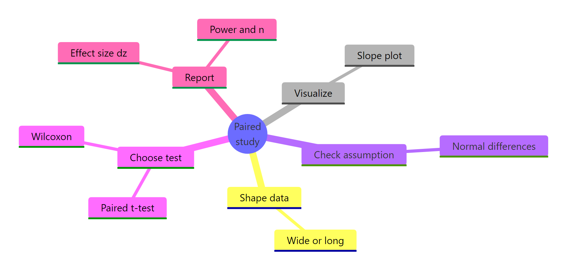
Figure 3: The full paired-analysis workflow at a glance.
The core habit to carry away: always analyze the differences, always report an effect size next to the p-value, and always pass your two columns as separate vectors because the formula interface will not take paired = TRUE.
References
- R Core Team. t.test: Student's t-Test (stats package documentation). Link
- R Core Team. wilcox.test: Wilcoxon Rank Sum and Signed Rank Tests. Link
- R Core Team. power.t.test: Power Calculations for Two-Sample t Test. Link
- R Core Team. shapiro.test: Shapiro-Wilk Normality Test. Link
- R Core Team. sleep: Student's Sleep Data. Link
- tidyr documentation. pivot_longer(). Link
- Wickham, H., Cetinkaya-Rundel, M., and Grolemund, G. R for Data Science, 2nd Edition. Link
- Wikipedia. Paired difference test. Link
Continue Learning
- t-Tests in R: all four t-test variants, including how the paired test fits alongside one-sample and two-sample tests.
- Wilcoxon Signed-Rank Test in R: the nonparametric partner for paired data, explained from scratch.
- Effect Size in R: Cohen's d and related measures for reporting how big an effect really is.
- Statistical Power Analysis in R: plan sample sizes before you collect data, for paired and unpaired designs.