Statistical vs Practical Significance in R
Statistical significance tells you an effect is probably real. Practical significance tells you whether it is big enough to care about. They are not the same, and mixing them up is one of the most expensive mistakes in data analysis. This tutorial uses base R throughout, so you need no extra packages.
What is the difference between statistical and practical significance?
Imagine your team tests a new checkout page against the old one and times how long each customer takes to check out. With 50,000 customers in each group, the test comes back "statistically significant." Before you celebrate, look at the numbers. The code below shows the trap in one shot: a rock-solid p-value sitting on top of a difference so small no customer would ever feel it.
We will simulate the two groups and run a standard t-test, which compares the average checkout time of the two pages and reports a p-value.
The p-value is 0.00118. That is far below the usual 0.05 cutoff, so by the textbook rule the new page is "significantly" faster. The walk-through: rnorm() drew 50,000 random checkout times for each page, t.test() compared their averages, and the tiny p-value says a gap this size is very unlikely to be pure chance.
Now ask the question the p-value never answers: how much faster? Let us look at the actual averages.
The new page saves about 0.2 seconds. Two tenths of one second, on a page that takes half a minute. No human would ever notice that. The result is statistically significant and practically meaningless at the same time.
That gap is the whole topic of this tutorial. Statistical significance answers "is this effect probably real, or could it be random noise?" You measure it with a p-value. Practical significance answers "is this effect big enough to change a decision?" You measure it with the size of the effect, not its p-value.
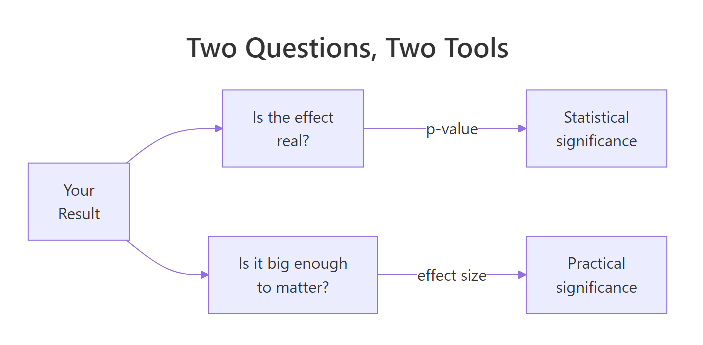
Figure 1: Two different questions, answered by two different tools.
Try it: Express the 0.2-second gap as a percentage of the current page's average time. A number this small tells you at a glance how trivial the improvement is.
Click to reveal solution
Explanation: The improvement is under 0.7 percent of the current checkout time. Dividing the raw gap by the baseline turns "0.2 seconds" into "basically nothing," which is exactly how a stakeholder would read it.
Why do large samples make almost everything statistically significant?
Here is the uncomfortable truth behind the checkout example: with a big enough sample, almost any difference becomes statistically significant, no matter how tiny. To see why, you only need to know what a t-test actually measures.
A t-test builds a t-statistic, and the p-value comes from that number. The formula is short: the t-statistic is the size of the effect divided by the standard error. The standard error shrinks as the sample grows, because more data means a more precise estimate. So even a frozen, tiny effect produces a bigger and bigger t-statistic as you collect more data, which drives the p-value down toward zero.
Let us prove it. We will hold the difference fixed at exactly 0.2 seconds and the spread fixed at 10, then change only the sample size and watch the p-value.
Read down the p_value column: 0.92, then 0.75, then 0.32, then 0.0016. The exact same 0.2-second difference goes from "nowhere near significant" to "highly significant" purely because the sample got bigger. Nothing about the effect changed. The walk-through: se falls as sizes rises, so t_stat climbs, and pt() converts that into an ever-smaller p-value.
Now read the cohens_d column, which measures the effect in standard-deviation units (the next section builds it from scratch). It sits at 0.02 the whole way down. The size of the effect never moved. Only your certainty that it is not exactly zero did.
Try it: Rerun the sweep, but change the frozen difference from 0.2 to 2 seconds. A ten-times-bigger effect should turn significant at a much smaller sample size.
Click to reveal solution
Explanation: A real 2-second effect reaches significance by n = 500, while the trivial 0.2-second effect needed n = 50,000. Bigger true effects need less data to detect, but a big enough sample eventually flags even the tiniest gap.
How do you measure practical significance with effect size?
If the p-value cannot tell you whether an effect is big, what can? The answer is effect size: a number that measures the gap in a way that does not inflate with sample size. The most common one for comparing two means is Cohen's d, which expresses the difference in standard-deviation units.
The idea is simple. Instead of asking "how many seconds apart are the two averages," Cohen's d asks "how many standard deviations apart are they." Dividing by the spread makes the number comparable across studies and, crucially, independent of how many people you tested.
You have already seen the concept above, so here is the formula it comes from. Skip it if you like; the code right after does the same arithmetic.
$$d = \frac{\bar{x}_1 - \bar{x}_2}{s_p}, \qquad s_p = \sqrt{\frac{(n_1-1)s_1^2 + (n_2-1)s_2^2}{n_1 + n_2 - 2}}$$
Where:
- $\bar{x}_1 - \bar{x}_2$ = the raw gap between the two group averages
- $s_p$ = the pooled standard deviation, the typical spread combined across both groups
- $n_1, n_2$ = the two sample sizes
- $s_1^2, s_2^2$ = the two group variances
Let us turn that formula into a small function and run it on the checkout data.
Cohen's d for the checkout test is 0.02. That is the same tiny number you saw in the sweep, and it does not care that we had 50,000 people per group. The walk-through: the function pools the two spreads into pooled_sd, then divides the raw mean gap by it, giving the effect in standard-deviation units.
How do you read a d of 0.02? Jacob Cohen offered rough benchmarks, still the most quoted starting point.
| Cohen's d | Rough label | What it feels like |
|---|---|---|
| 0.20 | Small | Detectable only with care |
| 0.50 | Medium | Visible to the naked eye |
| 0.80 | Large | Obvious, hard to miss |
At 0.02, the checkout effect is far below even "small." Now contrast that with an effect that genuinely matters: a drug trial where the treatment lifts a score by 12 points.
Here the p-value is tiny (0.0000013) and the effect size is large (d = 0.93). This is what you want: a result that is both real and big. The walk-through: t.test()$p.value pulls out just the p-value, and cohens_d() reports a gap of nearly one full standard deviation, which lands well past Cohen's "large" mark.
Try it: A tutoring program is tested on 40 students before and after. Compute Cohen's d for the improvement using the cohens_d() function you just wrote.
Click to reveal solution
Explanation: The tutoring program has a Cohen's d of 0.61, a medium-to-large effect. Unlike a p-value, this number would read the same whether the class had 40 students or 40,000.
How do confidence intervals show practical significance?
Effect size gives you one number for the gap. A confidence interval gives you something even more useful: the plausible range for the true effect. If the entire range is trivially small, the effect is trivially small, even when the p-value is far below 0.05.
A 95 percent confidence interval is the band of values that are consistent with your data. The t-test already computed one for the checkout gap. Let us pull it out on its own.
The interval runs from 0.08 to 0.33 seconds. Two things jump out. First, it does not include zero, which is another way of seeing the result is statistically significant. Second, and more important, even the most optimistic end of the range is a third of a second. The best case is still nothing a customer would feel. The walk-through: $conf.int extracts the two bounds, and both sit far below anything a person would notice.
Compare that to the drug trial, where the interval tells a very different story.
The drug's interval runs from about 8 to 18 points. Even the worst case, an 8-point lift, is a meaningful improvement. The interval is not just away from zero; it is entirely inside "this matters" territory. That is practical significance you can see at a glance.
Try it: Pull the lower and upper bounds of the drug interval into separate values using square-bracket indexing. The interval is just a length-two vector.
Click to reveal solution
Explanation: A confidence interval is an ordinary vector, so ex_ci[1] and ex_ci[2] grab its two ends. Being able to read both bounds is what lets you judge the effect's size, not just its significance.
How do you decide what counts as practically significant?
So far we have judged effects loosely: 0.2 seconds feels trivial, 12 points feels real. That gut feeling is not good enough for a real decision. The fix is to set a threshold before you run the test: the smallest effect that would actually change what you do. Researchers call this the smallest effect size of interest, or SESOI.
Setting the threshold up front stops you from rationalizing whatever result you happen to get. For the checkout page, suppose the team agrees in advance: a redesign is only worth shipping if it saves at least 3 seconds. Now the decision becomes mechanical. Compare the observed effect, and its whole confidence interval, against that 3-second line.
The observed saving is 0.204 seconds and even the top of the confidence interval is 0.327 seconds. Both sit far below the 3-second threshold, so ci_upper < threshold returns TRUE. The verdict: statistically significant, but not practically significant. Do not ship it. The walk-through: we take the absolute effect and the largest plausible effect, then check that even the best case falls short of the line the team drew.
Every result lands in one of four boxes, depending on the two questions. The chart below maps them out.
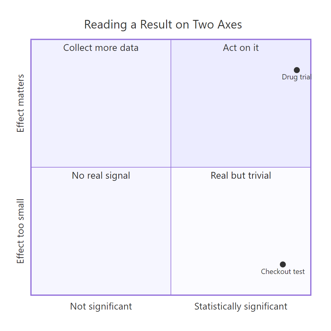
Figure 2: Every result sits somewhere on these two axes.
The dangerous box is the bottom-right: statistically significant but practically trivial. That is where huge samples push almost everything, and where the checkout test landed.
Try it: Apply the same threshold logic to the drug trial. If the team only cares about improvements of at least 5 points, check whether even the smallest plausible effect clears that bar.
Click to reveal solution
Explanation: Even the most pessimistic plausible effect, 7.99 points, clears the 5-point threshold. So the drug is both statistically and practically significant: the whole confidence interval sits above what the team cares about.
Complete Example: A/B Test Decision From Start to Finish
Let us put every piece together on the kind of test a real company runs. Your site gets heavy traffic, so an experiment collects 2,000,000 visitors per variant. You are testing whether a new landing page lifts the signup rate above the current 12.0 percent. The new page truly converts a hair better, at 12.1 percent. With traffic this large, the test will be significant. The real question is whether a hair is worth shipping.
First, simulate the two variants and run a proportion test, which compares two conversion rates.
The p-value is 0.01722, comfortably under 0.05. The new page is statistically significantly better. If you stopped here, you would ship it. But you know better now, so measure the size of the win.
The lift is 0.0775 percentage points, and the confidence interval says the true lift is somewhere between 0.014 and 0.14 percentage points. Even the optimistic end, 0.14 points, means fewer than 3 extra signups per 2,000 visitors. The walk-through: we convert the raw counts into rates, take the difference as a percentage point lift, and rescale the test's interval into the same units so it is easy to read.
Now make the call with a pre-set threshold. Suppose the product team decided beforehand that a redesign has to lift signups by at least 0.5 percentage points to justify the engineering and risk. The entire confidence interval, top included, is below 0.5. So the honest decision is: significant, yes, but do not ship. The win is too small to be worth the cost.
Practice Exercises
These combine the ideas above. Try each before opening the solution. The exercises use their own variable names, so they will not disturb the earlier examples.
Exercise 1: Significant is not the only question
Two teaching methods are compared on 80 students each. Run a t-test to check statistical significance, then compute Cohen's d. What do you conclude when the p-value and the effect size seem to disagree?
Click to reveal solution
Explanation: The p-value is 0.1086, above 0.05, so the difference is not statistically significant. Yet Cohen's d is 0.255, a real small-to-medium effect. The two do not actually disagree: with only 80 students the study is underpowered, so a genuine effect fails to reach significance. Not significant does not mean no effect; it can mean not enough data.
Exercise 2: Find where a trivial effect turns significant
A frozen effect of d = 0.1 is tested at growing sample sizes. Using the same deterministic approach from the sweep earlier, find the smallest sample size in the list where the p-value drops below 0.05. Confirm the effect size never changes.
Click to reveal solution
Explanation: The p-value crosses 0.05 between n = 500 and n = 1000; by n = 1000 it is 0.0255. The effect size stayed frozen at d = 0.1 the whole time. Significance was bought with sample size, not with a bigger effect.
Exercise 3: The full workflow on one result
An ed-tech company tests a new app feature on 10,000 students and measures test scores. Run the complete practical-significance workflow: get the p-value, the effect size, and the confidence interval, then decide against a threshold of 2 points (the smallest score gain the company would act on).
Click to reveal solution
Explanation: The result is statistically significant (p = 0.00087) but the effect is negligible: Cohen's d is 0.047 and the whole confidence interval, 0.23 to 0.90 points, sits below the 2-point threshold. The feature raises scores by well under a point. Significant, but not worth acting on.
Summary
Statistical significance and practical significance answer two different questions, and a good analysis reports both. The table below is your quick reference.
| Concept | Question it answers | Tool in R |
|---|---|---|
| Statistical significance | Is the effect probably real? | t.test(), prop.test() p-value |
| Practical significance | Is the effect big enough to matter? | Cohen's d, effect size |
| Plausible range | How big could the true effect be? | t.test()$conf.int |
| Decision rule | Does it clear my threshold? | Compare effect and interval to a pre-set SESOI |
The one habit that keeps you out of trouble: never read a p-value on its own. Pair it with an effect size and a confidence interval, and judge both against a threshold you set before seeing the data. The mindmap below recaps the whole picture.
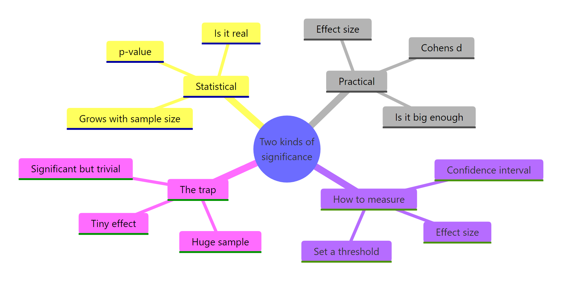
Figure 3: The whole picture at a glance.
Key takeaways:
- A small p-value means "unlikely to be chance," not "big enough to matter."
- Large samples make almost any difference statistically significant, so significance alone is a weak signal.
- Effect size (like Cohen's d) measures the magnitude of an effect and does not inflate with sample size.
- A confidence interval shows both significance and magnitude at once; read the whole interval, not just whether it excludes zero.
- Decide with a threshold set in advance, ideally from real-world costs and benefits rather than a generic benchmark table.
Frequently Asked Questions
A few questions come up again and again once people see the gap between the two kinds of significance. Here are quick answers.
Can a result be practically significant but not statistically significant?
Yes. A real, meaningful effect measured in a small or underpowered study can easily miss the p < 0.05 cutoff, exactly as you saw in Exercise 1. That is why you report the effect size and confidence interval too: they reveal a genuine effect that a p-value alone would let you dismiss as "not significant."
Is a p-value of 0.001 more practically significant than a p-value of 0.04?
No. A smaller p-value means you are more confident the effect is not exactly zero, not that the effect is bigger. Two results with wildly different p-values can have identical effect sizes. Practical size comes from the effect size and confidence interval, never from how small the p-value is.
What effect size should I use for two proportions instead of two means?
For two means, Cohen's d is the standard choice. For two proportions, the most decision-relevant number is usually the plain difference in rates, measured in percentage points, together with its confidence interval, as in the complete example above. Cohen's h is a standardized alternative when you need one comparable across studies.
How do I choose the smallest effect size of interest?
Set it from real-world costs and benefits whenever you can: the smallest improvement that would actually change your decision, given what the change costs. A generic benchmark table is only a last resort. Ask "how big would the effect have to be for us to act?" and use that number as your threshold, decided before you see the data.
Does a larger sample size make my results more practically significant?
No. A larger sample makes tiny effects easier to detect statistically, but it does not change how big the effect actually is. If anything, a very large sample widens the gap between statistical and practical significance, because it will flag effects far too small to matter.
References
- Sullivan, G. M. & Feinn, R. (2012). Using Effect Size, or Why the P Value Is Not Enough. Journal of Graduate Medical Education. Link. The short paper this whole tutorial builds on: why a p-value alone never tells you if an effect matters.
- Lakens, D. (2013). Calculating and reporting effect sizes to facilitate cumulative science. Frontiers in Psychology. Link. A practical how-to for computing and reporting Cohen's d and other effect sizes.
- Lakens, D., Scheel, A. M. & Isager, P. M. (2018). Equivalence Testing for Psychological Research: A Practical Primer. Advances in Methods and Practices in Psychological Science. Link. Introduces equivalence testing, the formal way to declare an effect too small to care about.
- R Core Team.
t.test{stats} reference manual. Link. Official docs for the function behind every p-value and confidence interval on this page. - R Core Team.
prop.test{stats} reference manual. Link. Official docs for comparing two proportions, as in the A/B test example. - Wikipedia. Effect size. Link. A broad catalogue of effect-size measures beyond Cohen's d.
- Wikipedia. Clinical significance (statistical vs practical significance). Link. The clinical framing of the same statistical-versus-practical distinction.
- R Core Team. An Introduction to R. Link. A refresher on the base-R basics this tutorial assumes.
Continue Learning
- Effect Size in R: go deeper into Cohen's d, eta-squared, and correlation-based effect sizes, the numbers that quantify practical significance.
- Hypothesis Testing in R: understand the framework that produces the p-value in the first place, so you know exactly what "significant" claims.
- Power Analysis in R: plan a sample size big enough to detect an effect that matters, instead of one so big it flags effects that do not.