Sampling Methods in R: Random, Stratified, Cluster
Sampling means measuring a small group so you can learn about a much larger group without surveying everyone. A sampling method is the rule you use to pick that small group. This guide covers the four methods you meet most often, simple random, systematic, stratified, and cluster, and shows you how to run each one in R, when to reach for it, and why the choice changes how good your answer is.
Everything below runs on a small employee population we build in the first code block, using base R and the dplyr package. You can run every block right here in the page and change the numbers to experiment. No files to download.
How do you draw a simple random sample in R?
The simplest fair way to pick a sample is to give every member of the group the same chance of being chosen. That is a simple random sample, and it is the baseline every other method is measured against. Let's build a small population of employees and draw one, so you can see the whole move in code before we name any of the parts.
The code below creates a data frame called company with 1000 employees. Each employee has a region, a team, and a satisfaction score from a survey. Then slice_sample() from dplyr picks 5 employees at random. Watch the output: it is 5 rows pulled from the 1000, with no pattern to who got picked.
Here is what just happened, line by line. set.seed(2026) fixes the random number generator so the population comes out the same for you as it did for me. rep() builds the region column: 500 in East, 300 in Central, 200 in West. rnorm() gives each person a satisfaction score that depends on their region. Then set.seed(1) resets the generator again, and slice_sample(company, n = 5) returns 5 randomly chosen rows.
The practical takeaway is that those 5 employees were chosen by pure chance. Nobody's satisfaction score, region, or team made them more or less likely to appear. That is the defining feature of a simple random sample, and it is why the sample tends to look like the population in miniature.
Base R has done this since long before dplyr existed. The sample() function picks random positions without replacement (no employee is picked twice), and you use those positions to subset the data. It gives you the same kind of result.
Notice the rows are identical to the dplyr version. That is not a coincidence. slice_sample() is a tidy wrapper around the same idea: pick random row positions, then return those rows. Use whichever style fits the rest of your code. We will lean on slice_sample() from here because it drops straight into a dplyr pipeline.
Often you want a fraction of the data rather than a fixed count. The prop argument does that. Here we take 10 percent of the 1000 employees, which is 100 people.
The prop = 0.10 argument means "give me 10 percent of the rows," so nrow() confirms 100 employees came back. Fixed count with n or a fraction with prop, both are simple random sampling. You just picked the size differently.
Try it: Draw a simple random sample of 8 employees from company and confirm the size with nrow(). Use slice_sample().
Click to reveal solution
Explanation: slice_sample(company, n = 8) returns 8 randomly chosen rows, and nrow() counts them. The set.seed() line just makes the draw repeatable.
What is systematic sampling, and how do you do it in R?
Simple random sampling needs a random draw for every unit you pick. Systematic sampling is a lighter-weight cousin: you line the population up in some order, pick one random starting point, then take every k-th unit from there. It is popular when items arrive in a stream, like every 20th product off a line or every 10th visitor through a door.
The step size k is the population size divided by the sample size. For 1000 employees and a target of 50, k is 20. You then pick a random start between 1 and 20 and grab positions like 10, 30, 50, and so on. The code computes the step, picks the start, and builds the row positions with seq().
Reading the output: the random start landed on position 10, so with a step of 20 we collected 50 rows. So this sample is employees at positions 10, 30, 50, and onward to 990. The only randomness was choosing where to start; everything after that is mechanical.
Because our population is ordered by region, taking every 20th person spreads the sample evenly across the whole ordered list. Let's check how the regions came out.
The systematic sample landed 25 East, 15 Central, 10 West employees. That matches the population split of 500, 300, 200 almost perfectly. When the ordering has no hidden pattern, systematic sampling behaves a lot like simple random sampling and costs less effort.
Try it: Draw a systematic sample of 100 employees. Work out the step k as nrow(company) %/% 100, pick a random start, then take every k-th row. Report the step and the number of rows.
Click to reveal solution
Explanation: A bigger sample means a smaller step. For 100 out of 1000 the step drops to 10, so you take every 10th employee.
How does stratified sampling work in R?
Sometimes you have subgroups you must represent no matter what, like regions or age bands. Stratified sampling guarantees it. You split the population into groups called strata, then draw a random sample inside each stratum. No stratum can be missed, because you sample from every one.
In dplyr this is a two-verb move. group_by(region) tells dplyr to treat each region separately, and slice_sample() then draws inside each group. The |> between the lines is the pipe: it feeds the result of each line into the next, so you read the steps top to bottom. The ungroup() at the end clears the grouping so later steps behave normally. Here we take 10 percent of each region.
Ten percent of each region gives 50 from East, 30 from Central, and 20 from West, for 100 in total. Because each region contributes the same fraction, the big regions send more people and the small ones send fewer. This is called proportional allocation, and it keeps the sample's group sizes in step with the population's.
Does the sample really mirror the population? Let's put the two side by side. prop.table(table(...)) turns raw counts into shares that add to 1.
The two rows are identical: 30 percent Central, 50 percent East, 20 percent West, in both the population and the sample. Proportional stratified sampling locks the group shares in place. A simple random sample would land close to these shares but wobble a little from draw to draw; stratifying removes that wobble.
You do not have to match the population shares. Sometimes you want the same number from each group, for example to compare regions on equal footing. That is equal allocation: just pass a fixed n instead of prop.
Now every region contributes exactly 30 people, even though West has far fewer employees than East. Equal allocation is great for comparing groups, but the sample no longer mirrors the population, so you would need to weight the groups back to their true sizes before making a population-wide estimate.
mutate() or summarise() silently keep running per region, which can produce puzzling results three steps downstream.The formula behind proportional allocation is short. If you want stratum h to get its fair share, set its sample size to the total sample size times the stratum's share of the population.
$$n_h = n \times \frac{N_h}{N}$$
Where:
- $n_h$ = how many to sample from stratum $h$
- $n$ = total sample size you want
- $N_h$ = number of people in stratum $h$ in the population
- $N$ = total population size
If you are not interested in the formula, skip it. Passing prop to slice_sample() does this arithmetic for you.
Try it: Draw a proportional stratified sample of 5 percent from each region and count how many came from each. Use group_by() and slice_sample(prop = ...).
Click to reveal solution
Explanation: Five percent of 300, 500, and 200 is 15, 25, and 10, so the sample keeps the region proportions exactly.
Why does stratified sampling give more precise estimates?
We keep saying stratified sampling is "more precise." Rather than assert it, let's measure it. Precision here means how much your estimate jumps around if you were to repeat the whole sampling process many times. A precise method gives nearly the same answer every time; a noisy one swings widely.
First, the target. The whole point of a sample is to estimate something about the population, so let's compute the true average satisfaction we are trying to hit.
The true average is 63.12. In real life you never get to see this number, which is exactly why you sample. Now we run a fair race. We draw 1000 simple random samples of 100 people, and 1000 proportional stratified samples of 100 people, and record the mean satisfaction each time. Then we compare how much each method's estimates spread out.
The standard deviation of the 1000 estimates is the spread we care about. Simple random sampling scattered its estimates with a standard deviation of 1.073, while stratified sampling scattered its estimates by only 0.762. A smaller number means the estimates cluster tighter around the truth. Let's express that as a percentage.
Stratifying cut the spread of the estimate by 29 percent, using the exact same sample size of 100. That is a free precision gain, bought only by organizing the draw by region instead of ignoring region.
Try it: The spread also shows up in the range. Compute the range (max minus min) of srs_means and of strat_means and compare. Use diff(range(...)).
Click to reveal solution
Explanation: Across 1000 samples, the simple random estimates spanned 6.55 points while the stratified estimates spanned only 4.99. The stratified method is steadier by every measure of spread.
What is cluster sampling, and how is it different from stratified?
Stratified and cluster sampling both start by splitting the population into groups, which makes them easy to confuse. The difference is what you do next. Stratified sampling draws a few units from every group. Cluster sampling picks a few whole groups at random and takes everyone inside them.
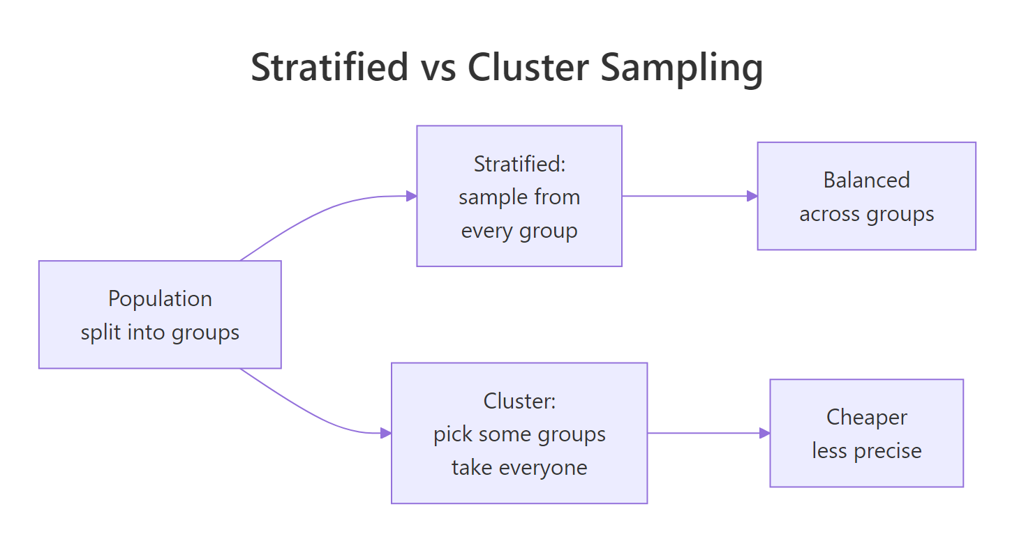
Figure 1: Stratified sampling draws from every group; cluster sampling picks whole groups and takes everyone in them.
You reach for cluster sampling when the groups are natural units that are expensive or slow to reach one by one, like schools or city blocks. It is far cheaper to visit 10 schools and survey everyone there than to chase 300 students scattered across 200 schools. In our data, teams are natural clusters. Let's pick 10 of the 50 teams at random and take every employee in them.
We selected 10 teams, and because every team has 20 people, that gave us 200 employees. The random draw was over teams, not people. Once a team was chosen, all 20 of its members came along automatically.
There is a catch, and it is the whole reason cluster sampling is different from stratified. Because we only visited 10 of the 50 teams, the regions can come out lopsided. Let's look.
Compare this to the population shares of 30 percent Central, 50 percent East, 20 percent West. The cluster sample came out 30, 40, 30 percent instead, over-representing West and under-representing East. Cluster sampling gives no guarantee that subgroups stay balanced, which is the opposite of what stratified sampling promises.
Try it: Draw a cluster sample of 5 teams and count how many people it contains. Use sample() to pick the teams, then filter().
Click to reveal solution
Explanation: Five teams of 20 give exactly 100 people. You chose 5 clusters at random and took all their members.
How do you choose the right sampling method?
You now have four tools. Picking between them comes down to two questions: are your natural groups costly to reach, and do you have subgroups you must represent? The guide below walks you through it.
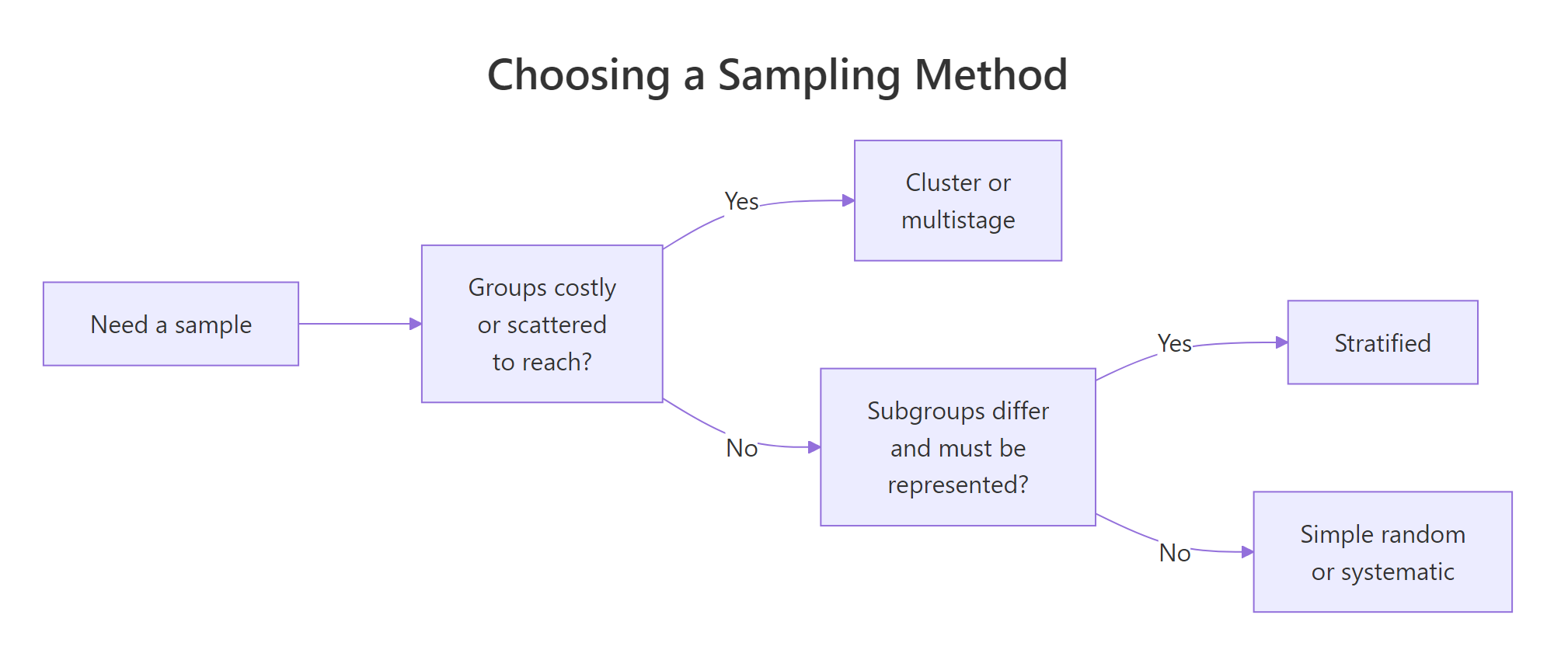
Figure 2: A quick decision guide for picking a sampling method.
Here is the same advice as a table you can scan, with the trade-off each method makes.
| Method | How it picks | Best when | Precision | Cost |
|---|---|---|---|---|
| Simple random | Every unit an equal chance | You have a clean list of everyone | Good | Higher |
| Systematic | Every k-th unit after a random start | Units arrive in a stream | Good, if no cycle | Low |
| Stratified | Sample within every subgroup | Subgroups differ and must be shown | Best | Medium |
| Cluster | Take whole groups at random | Groups are costly or scattered to reach | Lower | Lowest |
Real surveys often combine these into multistage sampling. You cluster first to save travel, then sample inside each chosen cluster instead of surveying everyone, which cuts cost twice. The code below does two stages: pick 8 teams, then sample 5 people from each of those teams.
Stage 1 chose 8 teams with sample(). Stage 2 grouped by team and drew 5 people from each with slice_sample(n = 5), for 40 people in all. You visit only 8 teams instead of all 50, and within each you talk to 5 people instead of all 20. That is a large saving in effort.
Try it: Build a two-stage sample that picks 6 teams and then 4 people from each. Report the number of teams and total people.
Click to reveal solution
Explanation: Six teams times 4 people each is 24 responses, gathered from only 6 site visits.
Complete Example
Let's put the pieces together in a task you might actually get: survey 100 of the 1000 employees, and make sure each region is represented in proportion to its size. This is proportional stratified sampling from start to finish.
First, plan the allocation. We count how many employees are in each region, then work out each region's share of 100.
The plan says survey 50 from East, 30 from Central, 20 from West. Since those are exactly 10 percent of each region, we can draw the survey by taking prop = 0.10 within each region, and the counts will match the plan.
The drawn sample matches the plan exactly: 50 East, 30 Central, 20 West. Now we use the survey to estimate the population's average satisfaction and attach a rough standard error, which measures how far off the estimate might be.
The survey estimated average satisfaction at 62.15, and the truth is 63.12. The estimate is within about one standard error of the real value, which is exactly the kind of accuracy a well-designed sample of 100 should give you. You learned the whole population's satisfaction by measuring one in ten employees, with the regions kept in balance the entire way.
Practice Exercises
These combine several ideas from the tutorial. Try each before opening the solution. The code uses my_ names so it will not clash with the tutorial's variables.
Exercise 1: Verify a stratified sample matches the population
Draw a proportional stratified sample of 15 percent from each region, then prove the sample's region shares match the population's shares. Build a two-row table of shares, one row for the population and one for the sample.
Click to reveal solution
Explanation: Proportional allocation forces the sample shares to equal the population shares, so both rows read 0.3, 0.5, 0.2. This is the guarantee stratified sampling gives you and simple random sampling does not.
Exercise 2: Measure the precision cost of cluster sampling
Run a small simulation to compare precision. Over 500 repeats, draw a simple random sample of 100 people and a cluster sample of 5 teams (also 100 people), record the mean satisfaction each time, and compare the standard deviation of the two sets of estimates. Which method is noisier?
Click to reveal solution
Explanation: With the same 100 people, cluster sampling scattered its estimates more than three times as widely as simple random sampling (3.485 versus 1.050). That is the precision you pay for the convenience of visiting only 5 teams.
Exercise 3: Estimate from a multistage sample
Draw a two-stage sample: pick 6 teams, then 8 people from each. Estimate the population's mean satisfaction from your 48 responses and compare it to the true mean of 63.12. Do not be surprised if it is off by a few points.
Click to reveal solution
Explanation: This draw estimated 67.79 against a truth of 63.12, a miss of about 4.7 points from just 48 people spread over 6 teams. That gap is the precision cost from Exercise 2 showing up in a single sample: fewer clusters means a noisier answer. More teams, or a larger sample, would tighten it.
Frequently Asked Questions
What is the difference between stratified and cluster sampling? Stratified sampling draws a few units from every group, so all groups are represented. Cluster sampling picks a few whole groups at random and takes everyone in them, so some groups are left out entirely. Use strata for balance and precision, clusters to save cost when groups are hard to reach.
Should I use slice_sample() or sample_n() and sample_frac()? Use slice_sample(). The older sample_n() and sample_frac() still work but have been superseded in modern dplyr, and slice_sample() covers both with the n and prop arguments.
Is systematic sampling a probability sample? Yes, as long as the starting point is chosen at random, every unit has a known chance of selection. The one thing to watch is periodicity: if the list repeats on a cycle equal to your step size, the sample can be biased, so shuffle the order when in doubt.
Do I always need set.seed()? Only when you want the exact same random draw again, which is useful for reproducible reports and for debugging. Set a seed before any random step. In a real one-off survey you can skip it, since you draw the sample once.
Does stratified sampling always beat simple random sampling? It helps most when the strata have different averages, as our regions do. If the groups are nearly identical on the thing you are measuring, stratifying adds effort for little precision gain. It never hurts precision, though, so it is a safe default when you have meaningful subgroups.
How large should my sample be? That depends on how precise you need the answer and how much the population varies. Sample size planning is its own topic, but the pattern you saw holds: bigger samples and smarter designs like stratification both shrink the spread of your estimate.
Summary
Sampling lets you answer questions about a large population by measuring a small slice of it. The method you pick decides how representative and how precise that slice is.
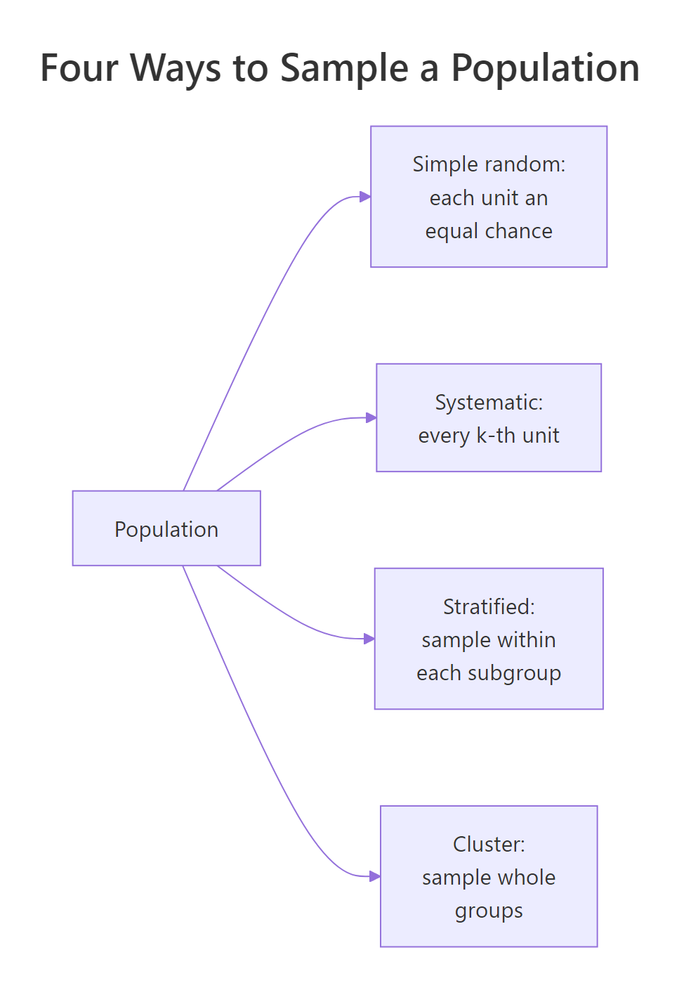
Figure 3: The four sampling methods at a glance, all starting from one population.
| Method | One-line how | Best when |
|---|---|---|
| Simple random | slice_sample(n =) or sample() picks at random |
You have a full list and want a fair baseline |
| Systematic | Every k-th unit after a random start | Units stream past in some order |
| Stratified | group_by() then slice_sample() inside each group |
You must represent subgroups and want precision |
| Cluster | sample() whole groups, then filter() to them |
Groups are costly or scattered to reach |
Key things to carry forward:
- Simple random sampling gives every unit an equal chance and is the baseline for everything else.
- Systematic sampling is cheaper but assumes the ordering has no hidden cycle.
- Stratified sampling represents every subgroup and tightened our estimate by 29 percent for free.
- Cluster sampling saves cost by taking whole groups, at the price of lower precision.
- Multistage sampling chains these together, most often clustering first, then sampling inside each cluster.
References
- dplyr documentation. slice_sample() and the slice family reference. The canonical docs for slice_sample() and its
n,prop, andweight_byarguments. Link - dplyr documentation. group_by() reference. Explains how grouping makes slice_sample() draw within each stratum. Link
- R Core Team. An Introduction to R, section on the sample() function. The base R sample() function used here for row positions and for picking clusters. Link
- Wickham, H., Cetinkaya-Rundel, M., and Grolemund, G. R for Data Science, 2nd Edition. A practical, beginner-friendly introduction to dplyr and the tidyverse workflow. Link
- Simple random sample. Wikipedia. A plain-language definition of simple random sampling and its properties. Link
- Stratified sampling. Wikipedia. Background on strata, proportional versus equal allocation, and the variance reduction. Link
- Cluster sampling. Wikipedia. More depth on the cost-precision trade-off and the design effect. Link
Continue Learning
- Populations, Samples and Sampling Bias in R: the why behind sampling, and how a bad sampling method quietly distorts your answer.
- Types of Data in Statistics: Categorical to Continuous: what kind of variable you are sampling shapes how you summarize it.
- What Statistics Is For: Questions, Evidence, Decisions: where sampling fits in the bigger job of learning from data.