scipy.signal.freqz

scipy.signal.freqz(b, a=1, worN=None, whole=False, plot=None)

Compute the frequency response of a digital filter.

Given the M-order numerator b and N-order denominator a of a digital filter, compute its frequency response:

            jw               -jw               -jwM
   jw    B(e  )  b[0] + b[1]e    + .... + b[M]e
H(e  ) = ---- = -----------------------------------
            jw               -jw               -jwN
         A(e  )  a[0] + a[1]e    + .... + a[N]e

Parameters:

b : array_like

Numerator of a linear filter. Must be 1D.

a : array_like

Denominator of a linear filter. Must be 1D.

worN : {None, int, array_like}, optional

If None (default), then compute at 512 frequencies equally spaced around the unit circle. If a single integer, then compute at that many frequencies. Using a number that is fast for FFT computations can result in faster computations (see Notes). If an array_like, compute the response at the frequencies given (in radians/sample; must be 1D).

whole : bool, optional

Normally, frequencies are computed from 0 to the Nyquist frequency, pi radians/sample (upper-half of unit-circle). If whole is True, compute frequencies from 0 to 2*pi radians/sample.

plot : callable

A callable that takes two arguments. If given, the return parameters w and h are passed to plot. Useful for plotting the frequency response inside freqz.

Returns:

w : ndarray

The normalized frequencies at which h was computed, in radians/sample.

h : ndarray

The frequency response, as complex numbers.

See also

freqz_zpk, sosfreqz

Notes

Using Matplotlib’s matplotlib.pyplot.plot function as the callable for plot produces unexpected results, as this plots the real part of the complex transfer function, not the magnitude. Try lambda w, h: plot(w, np.abs(h)).

A direct computation via (R)FFT is used to compute the frequency response when the following conditions are met:

1. An integer value is given for worN.
2. worN is fast to compute via FFT (i.e., next_fast_len(worN) equals worN).
3. The denominator coefficients are a single value (a.shape[0] == 1).
4. worN is at least as long as the numerator coefficients (worN >= b.shape[0]).

For long FIR filters, the FFT approach can have lower error and be much faster than the equivalent direct polynomial calculation.

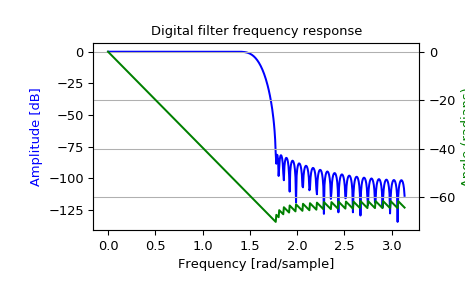
Examples

>>> from scipy import signal
>>> b = signal.firwin(80, 0.5, window=('kaiser', 8))
>>> w, h = signal.freqz(b)

>>> import matplotlib.pyplot as plt
>>> fig = plt.figure()
>>> plt.title('Digital filter frequency response')
>>> ax1 = fig.add_subplot(111)

>>> plt.plot(w, 20 * np.log10(abs(h)), 'b')
>>> plt.ylabel('Amplitude [dB]', color='b')
>>> plt.xlabel('Frequency [rad/sample]')

>>> ax2 = ax1.twinx()
>>> angles = np.unwrap(np.angle(h))
>>> plt.plot(w, angles, 'g')
>>> plt.ylabel('Angle (radians)', color='g')
>>> plt.grid()
>>> plt.axis('tight')
>>> plt.show()