scipy.signal.freqz_zpk

scipy.signal.freqz_zpk(z, p, k, worN=None, whole=False)

Compute the frequency response of a digital filter in ZPK form.

Given the Zeros, Poles and Gain of a digital filter, compute its frequency response:

:math:`H(z)=k \prod_i (z - Z[i]) / \prod_j (z - P[j])`

where \(k\) is the gain, \(Z\) are the zeros and \(P\) are the poles.

Parameters:

z : array_like

Zeroes of a linear filter

p : array_like

Poles of a linear filter

k : scalar

Gain of a linear filter

worN : {None, int, array_like}, optional

If single integer (default 512, same as None), then compute at worN frequencies equally spaced around the unit circle. If an array_like, compute the response at the frequencies given (in radians/sample).

whole : bool, optional

Normally, frequencies are computed from 0 to the Nyquist frequency, pi radians/sample (upper-half of unit-circle). If whole is True, compute frequencies from 0 to 2*pi radians/sample.

Returns:

w : ndarray

The normalized frequencies at which h was computed, in radians/sample.

h : ndarray

The frequency response.

See also

freqs

Compute the frequency response of an analog filter in TF form

freqs_zpk

Compute the frequency response of an analog filter in ZPK form

freqz

Compute the frequency response of a digital filter in TF form

Notes

Examples

>>> from scipy import signal
>>> z, p, k = signal.butter(4, 0.2, output='zpk')
>>> w, h = signal.freqz_zpk(z, p, k)

>>> import matplotlib.pyplot as plt
>>> fig = plt.figure()
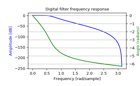
>>> plt.title('Digital filter frequency response')
>>> ax1 = fig.add_subplot(111)

>>> plt.plot(w, 20 * np.log10(abs(h)), 'b')
>>> plt.ylabel('Amplitude [dB]', color='b')
>>> plt.xlabel('Frequency [rad/sample]')

>>> ax2 = ax1.twinx()
>>> angles = np.unwrap(np.angle(h))
>>> plt.plot(w, angles, 'g')
>>> plt.ylabel('Angle (radians)', color='g')
>>> plt.grid()
>>> plt.axis('tight')
>>> plt.show()