Polygons from a reference map

This is pure annotation, so does not affect position scales.

geom_map(mapping = NULL, data = NULL, stat = "identity", ..., map,
  na.rm = FALSE, show.legend = NA, inherit.aes = TRUE)

Arguments

mapping	Set of aesthetic mappings created by aes or aes_. If specified and inherit.aes = TRUE (the default), it is combined with the default mapping at the top level of the plot. You must supply mapping if there is no plot mapping.
data	The data to be displayed in this layer. There are three options: If NULL, the default, the data is inherited from the plot data as specified in the call to ggplot. A data.frame, or other object, will override the plot data. All objects will be fortified to produce a data frame. See fortify for which variables will be created. A function will be called with a single argument, the plot data. The return value must be a data.frame., and will be used as the layer data.
stat	The statistical transformation to use on the data for this layer, as a string.
...	other arguments passed on to layer. These are often aesthetics, used to set an aesthetic to a fixed value, like color = "red" or size = 3. They may also be parameters to the paired geom/stat.
map	Data frame that contains the map coordinates. This will typically be created using fortify on a spatial object. It must contain columns x or long, y or lat, and region or id.
na.rm	If FALSE, the default, missing values are removed with a warning. If TRUE, missing values are silently removed.
show.legend	logical. Should this layer be included in the legends? NA, the default, includes if any aesthetics are mapped. FALSE never includes, and TRUE always includes.
inherit.aes	If FALSE, overrides the default aesthetics, rather than combining with them. This is most useful for helper functions that define both data and aesthetics and shouldn't inherit behaviour from the default plot specification, e.g. borders.

Aesthetics

geom_map understands the following aesthetics (required aesthetics are in bold):

• map_id

• alpha

• colour

• fill

• group

• linetype

• size

Examples

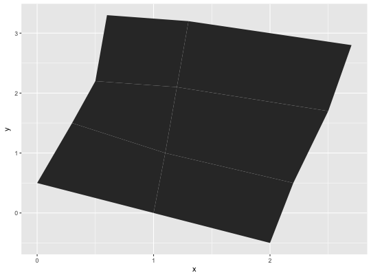
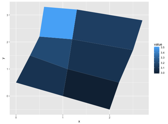
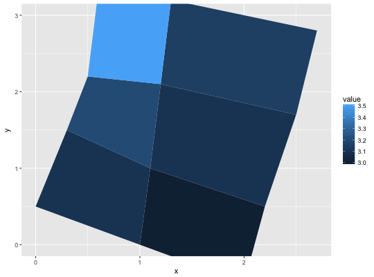
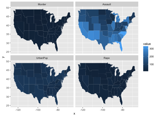
# When using geom_polygon, you will typically need two data frames:
# one contains the coordinates of each polygon (positions),  and the
# other the values associated with each polygon (values).  An id
# variable links the two together

ids <- factor(c("1.1", "2.1", "1.2", "2.2", "1.3", "2.3"))

values <- data.frame(
  id = ids,
  value = c(3, 3.1, 3.1, 3.2, 3.15, 3.5)
)

positions <- data.frame(
  id = rep(ids, each = 4),
  x = c(2, 1, 1.1, 2.2, 1, 0, 0.3, 1.1, 2.2, 1.1, 1.2, 2.5, 1.1, 0.3,
  0.5, 1.2, 2.5, 1.2, 1.3, 2.7, 1.2, 0.5, 0.6, 1.3),
  y = c(-0.5, 0, 1, 0.5, 0, 0.5, 1.5, 1, 0.5, 1, 2.1, 1.7, 1, 1.5,
  2.2, 2.1, 1.7, 2.1, 3.2, 2.8, 2.1, 2.2, 3.3, 3.2)
)

ggplot(values) +
  geom_map(aes(map_id = id), map = positions) +
  expand_limits(positions)
ggplot(values, aes(fill = value)) +
  geom_map(aes(map_id = id), map = positions) +
  expand_limits(positions)
ggplot(values, aes(fill = value)) +
  geom_map(aes(map_id = id), map = positions) +
  expand_limits(positions) + ylim(0, 3)

# Better example
crimes <- data.frame(state = tolower(rownames(USArrests)), USArrests)
crimesm <- reshape2::melt(crimes, id = 1)
if (require(maps)) {
  states_map <- map_data("state")
  ggplot(crimes, aes(map_id = state)) +
    geom_map(aes(fill = Murder), map = states_map) +
    expand_limits(x = states_map$long, y = states_map$lat)

  last_plot() + coord_map()
  ggplot(crimesm, aes(map_id = state)) +
    geom_map(aes(fill = value), map = states_map) +
    expand_limits(x = states_map$long, y = states_map$lat) +
    facet_wrap( ~ variable)
}