|
Observation Preprocessing
The goal of this session is to generate the observation input (i.e. the y0 shown in the WRFDA flowchart) for running WRFDA with conventional observations.
Reference: Download the tutorial presentation
OBSPROC for 3DVAR
Source code
Copy the pre-compiled code to your main working directory (/classroom/users/${USER}/DA), if you have not done so.
WRFDA/var/obsproc/obsproc.exe is the executable that will be used in this session.
Create your working directory
We recommend running each session in a separate directory, so that it will be easier to check for the necessary input files and look for what output files are created after a successful run.
For this exercise you should create /classroom/users/${USER}/DA/obsproc and use this as your working directory for this session.
mkdir -p /classroom/users/${USER}/DA/obsproc
cd /classroom/users/${USER}/DA/obsproc
Input data
- observations in little_r format
The first step of observation preprocessing is to prepare observations in little_r format.
For this tutorial, an observation file in little_r format is provided.
cp /classroom/wrfhelp/DATA/WRFDA/CONUS60/ob/2008020512/obs.2008020512 .
obs.2008020512 is the observation file for this exercise in little_r format. It is a text file; you can use emacs, vi, or another text editor to see its contents. For your own applications, you will have to prepare your own observation file.
- observation error table
The observation error file (obserr.txt) is provided with the WRFDA package under the var/obsproc directory.
Make sure it is present in your obsproc working directory.
ln -fs /classroom/users/${USER}/DA/WRFDA/var/obsproc/obserr.txt ./obserr.txt
- namelist.obsproc
For your reference, an example namelist (namelist.obsproc.3dvar.wrfvar-tut) has been included in the WRFDA package under var/obsproc directory.
Copy and rename the namelist to "namelist.obsproc" under your working directory.
cp /classroom/users/${USER}/DA/WRFDA/var/obsproc/namelist.obsproc.3dvar.wrfvar-tut ./namelist.obsproc
namelist.obsproc contains options to configure the little_r observation file location, domain, time window, etc.
For this tutorial case, you shouldn't need to change any settings in the namelist, but you should check the important settings to gain familiarity with the setup of OBSPROC. &record1 specifies information about your input file names, &record2 specifies date/time information, and &record7 and &record8 specify information about your domain. You can use emacs, vi, or nano for viewing and editing text files on the command line.
> vi namelist.obsproc
&record1
obs_gts_filename = 'obs.2008020512',
obs_err_filename = 'obserr.txt',
/
&record2
time_window_min = '2008-02-05_11:00:00',
time_analysis = '2008-02-05_12:00:00',
time_window_max = '2008-02-05_13:00:00',
/
...
&record7
IPROJ = 1,
PHIC = 40.00001,
XLONC = -95.0,
TRUELAT1= 30.0,
TRUELAT2= 60.0,
MOAD_CEN_LAT = 40.00001,
STANDARD_LON = -95.00,
/
&record8
IDD = 1,
MAXNES = 1,
NESTIX = 60, 200, 136, 181, 211,
NESTJX = 90, 200, 181, 196, 211,
DIS = 60, 10., 3.3, 1.1, 1.1,
NUMC = 1, 1, 2, 3, 4,
NESTI = 1, 40, 28, 35, 45,
NESTJ = 1, 60, 25, 65, 55,
/
...
Alternatively, rather than copying the observation file to your working directory, you can set obs_gts_filename to the full path of the file's location.
Run obsproc (obsproc.exe)
It is convenient to link the executable to your current working directory.
ln -sf /classroom/users/${USER}/DA/WRFDA/var/obsproc/obsproc.exe .
./obsproc.exe
On the classroom computers, running this step should take less than a minute.
Check output
A successful run of obsproc should result in lines similar to these near the end of the output on screen:
Write 3DVAR GTS observations in file obs_gts_2008-02-05_12:00:00.3DVAR (WRFDA V3.9)
Wrote 31140 lines of data in file: obs_gts_2008-02-05_12:00:00.3DVAR
No SSMI observations available.
STOP 99999
NOTE: If you see a message stating "The following floating-point exceptions are signalling" or similar, this is normal and can be safely ignored. |
Look for obs_gts_2008-02-05_12:00:00.3DVAR in your working directory. That is the main output from obsproc. You can open it using a text editor to check its content; it should look similar to this.
*.diag are diagnostic files. The writing of these files are controlled by the namelist settings under &record5. You should see (among other files):
- obs_duplicate_loc.diag: contains info about stations with multiple observations of the same type within your specified time window. For 3DVAR, if there are multiple observations of the same type at the same location, only one will be kept.
- obs_gts_read.diag: lists every observation read from the LITTLE_R input file, followed by a note if it was rejected due to being outside of the specified domain or outside the specified time window.
- obs_qc1.diag: first set of quality control checks: looks for and attempts to correct temperature and wind spikes as well as super-adiabatic conditions in sounding observations
- obs_qc2.diag: second set of quality control checks: looks for observations above the specified model top
- obs_recover_height.diag and obs_recover_pressure.diag: lists observations where missing height or pressure was recovered from other observed variables combined with the reference state
- obs_uncomplete.diag: remove observations that consist only of missing data
HEIGHT.txt, PRES.txt, RH.txt, SPD.txt, TEMP.txt, and UV.txt are observation errors in plain-text format for easy reference. Most names are self-explanatory. However, since some wind observations are of wind speed/direction while others are of the wind's U- and V-components, there are multiple files for wind errors. DIR.txt and SPD.txt are used for wind direction and speed errors respectively, while UV.txt is for U- and V-wind component errors.
Graphics
You can use an NCL script, provided at /classroom/wrfhelp/DATA/WRFDA/TOOLS/graphics/ncl/plot_ob_ascii_loc.ncl, to see the locations of observations contained in obs_gts_2008-02-05_12:00:00.3DVAR
cp /classroom/wrfhelp/DATA/WRFDA/TOOLS/graphics/ncl/plot_ob_ascii_loc.ncl .
Edit plot_ob_ascii_loc.ncl to provide the date, filenames and options of your case.
......
date = "2008020512"
obfile = "obs_gts_2008-02-05_12:00:00.3DVAR"
fgfile = "/classroom/wrfhelp/DATA/WRFDA/CONUS60/rc/2008020512/wrfinput_d01" ; for retrieving mapping info
out_type = "pdf"
plotname = "./obsloc"+date
......
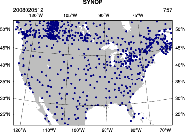
Run the NCL script
ncl plot_ob_ascii_loc.ncl
View the plot using display. Use spacebar to scroll through the plots of different observation types.
display obsloc2008020512.pdf
|
 |
OBSPROC for 4DVAR
So far we have prepared observations for 3DVAR: this method assumes all observations are at the same time, so all observations are contained within a single file. We can also prepare observations for 4DVAR, which is a method by which observations are assimilated at their actual time. You will learn more about this method in later lectures and exercises.
Prepare observations for 4DVAR
Now we will use OBSPROC to create ASCII observation files for a later 4DVAR exercise. Create /classroom/users/${USER}/DA/obsproc_4dvar and use this as your working directory.
mkdir /classroom/users/${USER}/DA/obsproc_4dvar
cd /classroom/users/${USER}/DA/obsproc_4dvar
As before, you will need an observation file in little_r format, an observation error table, and a namelist file.
This time, try creating your own "namelist.obsproc" from scratch. You'll need to set the following settings for this test case:
> vi namelist.obsproc
&record1
obs_gts_filename = '/classroom/wrfhelp/DATA/WRFDA/4dvar/ob/2017070400/obs.2017070400',
obs_err_filename = 'obserr.txt',
/
&record2
time_window_min = '2017-07-04_00:00:00',
time_analysis = '2017-07-04_03:00:00',
time_window_max = '2017-07-04_03:00:00',
/
&record3
max_number_of_obs = 400000,
/
&record4
domain_check_h = .true.,
/
&record5
/
&record6
ptop = 5000.0,
base_pres = 100000.0,
base_temp = 290.0,
base_lapse = 50.0,
base_strat_temp = 215.0,
base_tropo_pres = 20000.0
/
&record7
IPROJ = 1,
PHIC = 30.,
XLONC = 130.0,
TRUELAT1= 20.0,
TRUELAT2= 40.0,
MOAD_CEN_LAT = 30.,
STANDARD_LON = 130.,
/
&record8
IDD = 1,
MAXNES = 1,
NESTIX = 51, 200, 136, 181, 211,
NESTJX = 51, 200, 181, 196, 211,
DIS = 60, 10., 3.3, 1.1, 1.1,
NUMC = 1, 1, 2, 3, 4,
NESTI = 1, 40, 28, 35, 45,
NESTJ = 1, 60, 25, 65, 55,
/
&record9
use_for = '4DVAR',
num_slots_past = 3,
num_slots_ahead = 0,
/
Note that this time, instead of copying the little_r observation file to our working directory, we specify its location in the namelist with "obs_gts_filename".
Use the same observation error file as you did for the previous exercise, then run obsproc:
ln -fs /classroom/users/${USER}/DA/WRFDA/var/obsproc/obserr.txt ./obserr.txt
ln -sf /classroom/users/${USER}/DA/WRFDA/var/obsproc/obsproc.exe .
./obsproc.exe
On the classroom computers, running this step should take less than a minute.
NOTE: If you see messages stating "WARNING: ERROR in read_measurements", this is normal and can be safely ignored. This simply indicates that an observation in the input file is formatted incorrectly, and is being skipped. |
This time, you should see several observation files in your working directory:
obs_gts_2017-07-04_00:00:00.4DVAR
obs_gts_2017-07-04_01:00:00.4DVAR
obs_gts_2017-07-04_02:00:00.4DVAR
obs_gts_2017-07-04_03:00:00.4DVAR
These are the output observation files from obsproc, one for each time window. You can open them using a text editor; they should look similar to this. Note that the off-hour observation files (i.e., not 00z, 06z, 12z, or 18z) have fewer observations, since many regular observations are only taken at those times.
You will also see the same *.diag diagnostic files as with the 3DVAR case. The only difference is there will now be 4 duplicate time log files rather than one, since we have specified 4 observation time windows.
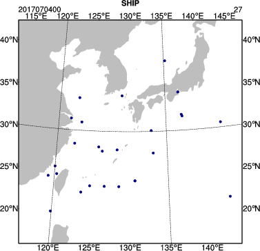
You can use the same NCL script as above (/classroom/wrfhelp/DATA/WRFDA/TOOLS/graphics/ncl/plot_ob_ascii_loc.ncl), to see the locations of observations contained in each of your observation files. Copy plot_ob_ascii_loc.ncl to your working directory, then edit it to provide the date, filenames and options for this case.
......
date = "2017070400"
obfile = "obs_gts_2017-07-04_00:00:00.4DVAR"; (or obs_gts_2017-07-04_01:00:00.4DVAR, obs_gts_2017-07-04_02:00:00.4DVAR, obs_gts_2017-07-04_03:00:00.4DVAR)
fgfile = "/classroom/wrfhelp/DATA/WRFDA/4dvar/rc/2017070400/wrfinput_d01" ; for retrieving mapping info
out_type = "pdf"
plotname = "./obsloc"+date
......
Run the NCL script, then view the output file (obsloc2017070400.pdf) using display. You should see plots similar to the one seen at right.
|
 |
OBSPROC for FGAT (First Guess at Appropriate Time)
Finally, let's look at a case where we prepare observations for FGAT, which stands for First Guess at Appropriate Time. This is a cheap method of 4D data assimilation, which gains some of the benefits of assimilating observations at their actual time without the expense of running full 4DVAR assimilation.
Prepare observations for FGAT
Now we will use OBSPROC to create ASCII observation files for FGAT, which will be used later in the 4D-ENVAR (4D-hybrid assimilation) exercise. Create /classroom/users/${USER}/DA/obsproc_fgat and use this as your working directory.
mkdir /classroom/users/${USER}/DA/obsproc_fgat
cd /classroom/users/${USER}/DA/obsproc_fgat
As before, you will need an observation file in little_r format, an observation error table, and a namelist file. This process is similar to the process for creating observation files for 4DVAR.
Again, try creating your own "namelist.obsproc" from scratch. You'll need to set the following settings for this test case:
> vi namelist.obsproc
&record1
obs_gts_filename = '/classroom/wrfhelp/DATA/WRFDA/hybrid/ob/2016012300/obs.2016012300',
obs_err_filename = 'obserr.txt',
/
&record2
time_window_min = '2016-01-22_21:00:00',
time_analysis = '2016-01-23_00:00:00',
time_window_max = '2016-01-23_03:00:00',
/
&record3
max_number_of_obs = 400000,
/
&record4
domain_check_h = .true.,
/
&record5
/
&record6
ptop = 5000.0,
base_pres = 100000.0,
base_temp = 290.0,
base_lapse = 50.0,
base_strat_temp = 215.0,
base_tropo_pres = 20000.0
/
&record7
IPROJ = 1,
PHIC = 35.,
XLONC = -75.0,
TRUELAT1= 20.0,
TRUELAT2= 40.0,
MOAD_CEN_LAT = 35.,
STANDARD_LON = -75.,
/
&record8
IDD = 1,
MAXNES = 1,
NESTIX = 111, 200, 136, 181, 211,
NESTJX = 111, 200, 181, 196, 211,
DIS = 24, 10., 3.3, 1.1, 1.1,
NUMC = 1, 1, 2, 3, 4,
NESTI = 1, 40, 28, 35, 45,
NESTJ = 1, 60, 25, 65, 55,
/
&record9
use_for = 'FGAT',
num_slots_past = 3,
num_slots_ahead = 3,
/
Use the same observation error file as you did for the previous exercises, then run obsproc:
ln -fs /classroom/users/${USER}/DA/WRFDA/var/obsproc/obserr.txt ./obserr.txt
ln -sf /classroom/users/${USER}/DA/WRFDA/var/obsproc/obsproc.exe .
./obsproc.exe
On the classroom computers, running this exercise should take about a minute.
Just as with 4DVAR, you should see several observation files in your working directory:
obs_gts_2016-01-22_21:00:00.FGAT
obs_gts_2016-01-22_22:00:00.FGAT
obs_gts_2016-01-22_23:00:00.FGAT
obs_gts_2016-01-23_00:00:00.FGAT
obs_gts_2016-01-23_01:00:00.FGAT
obs_gts_2016-01-23_02:00:00.FGAT
obs_gts_2016-01-23_03:00:00.FGAT
These are the output observation files from obsproc, one for each time window. You can open them using a text editor; they should look similar to this. Again, note that the off-hour observation files have fewer observations: obs_gts_2016-01-23_00:00:00.FGAT has more than 7000 observations, yet obs_gts_2016-01-22_23:00:00.FGAT has less than 1000!
You will also see the same *.diag diagnostic files as with the 3DVAR and 4DVAR cases. Since we have 7 time windows, some of the diagnostics will have 7 different files; one for each time.
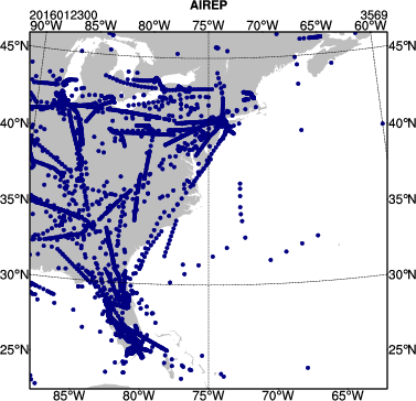
You can use the same NCL script as above (/classroom/wrfhelp/DATA/WRFDA/TOOLS/graphics/ncl/plot_ob_ascii_loc.ncl), to see the locations of observations contained in each of your observation files. Copy plot_ob_ascii_loc.ncl to your working directory, then edit it to provide the date, filenames and options for this case.
......
date = "2016012300"
obfile = "obs_gts_2016-01-23_00:00:00.FGAT"; (or obs_gts_2016-01-22_21:00:00.FGAT, obs_gts_2016-01-22_22:00:00.FGAT, etc.)
fgfile = "/classroom/wrfhelp/DATA/WRFDA/hybrid/fc/2016012300/wrfout_d01_2016-01-23_00:00:00.mean" ; for retrieving mapping info
out_type = "pdf"
plotname = "./obsloc"+date
......
Run the NCL script, then view the output file (obsloc2016012300.pdf) using display. You should see plots similar to the one seen at right.
|
 |
If you were successful, then congratulations, you are done with the basic OBSPROC exercise! If you still have additional time, you can move on to try compiling the WRFDA code yourself, or you can move on to additional practice below:
Additional practice
Reference the tutorial presentation and the User's Guide for instructions on the exercises below:
- Try modifying some of the settings under &record2 and &record9 to see how it changes the observations that are printed out.
- Set up any other domain of your interest, or some domains you have used for WRF practice. Use the command "ncdump -h" on any WRF file to find out the appropriate domain settings.
Take a look at WRFDA/var/obsproc/README.namelist to get some ideas on the options available for setting up your own domain.
|