#Non-parametric tests

All the previous tests assume that the data have different characteristics, such as normal distribution and homogeneity of variance. If the data CANNOT comply with these assumptions then the previous tests should not be used and alternative tests have to be explored. One set of tests are known as “Non-Parametric tests” or “Distribution Free Tests”.

Most of these tests do no use the original data but use the Ranks of the data. That is is done by assigning “new values” to the original data. The lowest value is assigned the rank of 1, the the next lowest value the rank of 2, and so on. Thus the highest value has the highest rank.

Then the analysis are on the ranks and NOT on the original values.

Los paquetes

#install.packages("car")
#install.packages("clinfun")
#install.packages("ggplot2")
#install.packages("pastecs")
#install.packages("pgirmess")

Activating packages

library(car)  # Companion to applied Regression
library(clinfun) # Clinical Trial Design and Data Analysis Functions
library(ggplot2) # Graphic production
library(pastecs) # Package for analysis of Space -Time ecological Series
library(pgirmess) # Spatial Analysis and Data Mining for Field Ecologist

## The legacy packages maptools, rgdal, and rgeos, underpinning the sp package,
## which was just loaded, will retire in October 2023.
## Please refer to R-spatial evolution reports for details, especially
## https://r-spatial.org/r/2023/05/15/evolution4.html.
## It may be desirable to make the sf package available;
## package maintainers should consider adding sf to Suggests:.
## The sp package is now running under evolution status 2
##      (status 2 uses the sf package in place of rgdal)

## Registered S3 method overwritten by 'pgirmess':
##   method   from
##   print.mc mc2d

## 
## Attaching package: 'pgirmess'

## The following object is masked from 'package:Rmisc':
## 
##     CI

Wilcoxon rank-sum test

The function “gl()” is a function that generates factors by specifying the pattern of their levels gl(n, k, lenght=n*k, labels=1:n, ordered=FALSE)

The hypothesis:

The level of depression posterior to the intake of alcohol is the same as those which take ecstasy.

Is this the null or alternate hipothesis?

The data come from 20 participants, 10 drinking alcohol and 10 taking ecstasy. Posterior to their consumption the “Beck Depression Inventory” was conducted on each of the participants. The scale is from 0 (happy) to 63 (truly depressed)

https://www.ismanet.org/doctoryourspirit/pdfs/Beck-Depression-Inventory-BDI.pdf

https://en.wikipedia.org/wiki/Beck_Depression_Inventory

Enter raw data

sundayBDI<-c(15, 35, 16, 18, 19, 
             17, 27, 16, 13, 20, 
             16, 15, 20, 15, 16, 
             13, 14, 19, 18, 18)
wedsBDI<-c(28, 35, 35, 24, 39, 32, 
           27, 29, 36, 35, 5, 6, 
           30, 8, 9, 7, 6, 17, 
           3, 10)
drug<-gl(2, 10, labels = c("Ecstasy", "Alcohol"))
Gender=gl(2, 10, labels = c("Male", "Female"))

drugData<-data.frame(Gender, drug, sundayBDI, wedsBDI)
drugData

## Warning in yaml::yaml.load(..., eval.expr = TRUE): NAs introduced by coercion:
## . is not a real

Gender	drug	sundayBDI	wedsBDI
Male	Ecstasy	15	28
Male	Ecstasy	35	35
Male	Ecstasy	16	35
Male	Ecstasy	18	24
Male	Ecstasy	19	39
Male	Ecstasy	17	32
Male	Ecstasy	27	27
Male	Ecstasy	16	29
Male	Ecstasy	13	36
Male	Ecstasy	20	35
Female	Alcohol	16	5
Female	Alcohol	15	6
Female	Alcohol	20	30
Female	Alcohol	15	8
Female	Alcohol	16	9
Female	Alcohol	13	7
Female	Alcohol	14	6
Female	Alcohol	19	17
Female	Alcohol	18	3
Female	Alcohol	18	10

Or Import the data

Exploratory analysis

library(readr)
Drug <- read_csv("Data_files_csv/Drug.csv")

## Rows: 20 Columns: 3
## ── Column specification ──────────
## Delimiter: ","
## chr (1): drug
## dbl (2): sundayBDI, wedsBDI
## 
## ℹ Use `spec()` to retrieve the full column specification for this data.
## ℹ Specify the column types or set `show_col_types = FALSE` to quiet this message.

head(Drug)

## Warning in yaml::yaml.load(..., eval.expr = TRUE): NAs introduced by coercion:
## . is not a real

drug	sundayBDI	wedsBDI
Ecstasy	15	28
Ecstasy	35	35
Ecstasy	16	35
Ecstasy	18	24
Ecstasy	19	39
Ecstasy	17	32

Descriptive statistics.

Note here we can use drugData[,c(2:3)], that we want the stats for column 2 and 3, and these be seperated by the drug (column 1).

NOTE the shapiro wilks test on the last line.

names(drugData)

## [1] "Gender"    "drug"      "sundayBDI" "wedsBDI"

by(drugData[,c(3:4)], drugData$drug, stat.desc, basic=TRUE, norm=TRUE)

## drugData$drug: Ecstasy
##                 sundayBDI     wedsBDI
## nbr.val       10.00000000  10.0000000
## nbr.null       0.00000000   0.0000000
## nbr.na         0.00000000   0.0000000
## min           13.00000000  24.0000000
## max           35.00000000  39.0000000
## range         22.00000000  15.0000000
## sum          196.00000000 320.0000000
## median        17.50000000  33.5000000
## mean          19.60000000  32.0000000
## SE.mean        2.08806130   1.5129074
## CI.mean.0.95   4.72352283   3.4224344
## var           43.60000000  22.8888889
## std.dev        6.60302961   4.7842334
## coef.var       0.33688927   0.1495073
## skewness       1.23571300  -0.2191665
## skew.2SE       0.89929826  -0.1594999
## kurtosis       0.26030385  -1.4810114
## kurt.2SE       0.09754697  -0.5549982
## normtest.W     0.81063991   0.9411413
## normtest.p     0.01952060   0.5657814
## ------------------------------------------------------------ 
## drugData$drug: Alcohol
##                 sundayBDI      wedsBDI
## nbr.val       10.00000000 1.000000e+01
## nbr.null       0.00000000 0.000000e+00
## nbr.na         0.00000000 0.000000e+00
## min           13.00000000 3.000000e+00
## max           20.00000000 3.000000e+01
## range          7.00000000 2.700000e+01
## sum          164.00000000 1.010000e+02
## median        16.00000000 7.500000e+00
## mean          16.40000000 1.010000e+01
## SE.mean        0.71802197 2.514182e+00
## CI.mean.0.95   1.62427855 5.687475e+00
## var            5.15555556 6.321111e+01
## std.dev        2.27058485 7.950542e+00
## coef.var       0.13845030 7.871823e-01
## skewness       0.11686189 1.500374e+00
## skew.2SE       0.08504701 1.091907e+00
## kurtosis      -1.49015904 1.079110e+00
## kurt.2SE      -0.55842624 4.043886e-01
## normtest.W     0.95946584 7.534665e-01
## normtest.p     0.77976459 3.933024e-03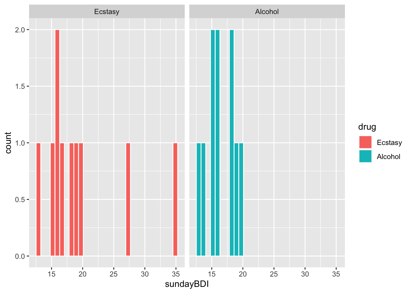

#shapiro.test(drugData$sundayBDI)  # this is to look at all the data, it is not the appropriate way to do the analisis of normality, why?
#shapiro.test(drugData$wedsBDI) # this is to look at all the data, it is not the appropriate way to do the analisis of normality, why?

Do a histogram by factor level for anxiety for Sunday.

library(ggplot2)

ggplot(drugData, aes(x=sundayBDI, fill=drug))+
  geom_histogram(colour="white")+
  facet_grid(~drug)

## `stat_bin()` using `bins = 30`.
## Pick better value with
## `binwidth`.

Test of equality of variance

This is one of the assumptions of parametric tests

#leveneTest(drugData$sundayBDI, drugData$drug, center = "mean")
leveneTest(drugData$sundayBDI, drugData$drug, center = "median")

## Warning in yaml::yaml.load(..., eval.expr = TRUE): NAs introduced by coercion:
## . is not a real

Df	F value	Pr(>F)
1	1.88	0.187
18

#leveneTest(drugData$wedsBDI, drugData$drug, center = "mean")
leveneTest(drugData$wedsBDI, drugData$drug, center = "median")

## Warning in yaml::yaml.load(..., eval.expr = TRUE): NAs introduced by coercion:
## . is not a real

Df	F value	Pr(>F)
1	0.0911	0.766
18

Wilcoxon rank-sum test

wilcox.test(x, y = NULL, alternative = c(“two.sided”, “less”, “greater”), mu = 0, paired = FALSE, exact = FALSE, correct = FALSE, conf.level = 0.95, na.action = na.exclude)

This is how to assing the Rank by Hand…… This is an example, the scripts will do this automatically.

Look for the smallest value……in the wedsBDI……

drugData$wedsRank=rank(drugData$wedsBDI)
drugData

## Warning in yaml::yaml.load(..., eval.expr = TRUE): NAs introduced by coercion:
## . is not a real

Gender	drug	sundayBDI	wedsBDI	wedsRank
Male	Ecstasy	15	28	12
Male	Ecstasy	35	35	17
Male	Ecstasy	16	35	17
Male	Ecstasy	18	24	10
Male	Ecstasy	19	39	20
Male	Ecstasy	17	32	15
Male	Ecstasy	27	27	11
Male	Ecstasy	16	29	13
Male	Ecstasy	13	36	19
Male	Ecstasy	20	35	17
Female	Alcohol	16	5	2
Female	Alcohol	15	6	3.5
Female	Alcohol	20	30	14
Female	Alcohol	15	8	6
Female	Alcohol	16	9	7
Female	Alcohol	13	7	5
Female	Alcohol	14	6	3.5
Female	Alcohol	19	17	9
Female	Alcohol	18	3	1
Female	Alcohol	18	10	8

Wilcoxon test: A non-parametric test

names(drugData)

## [1] "Gender"    "drug"      "sundayBDI" "wedsBDI"   "wedsRank"

head(drugData)

## Warning in yaml::yaml.load(..., eval.expr = TRUE): NAs introduced by coercion:
## . is not a real

Gender	drug	sundayBDI	wedsBDI	wedsRank
Male	Ecstasy	15	28	12
Male	Ecstasy	35	35	17
Male	Ecstasy	16	35	17
Male	Ecstasy	18	24	10
Male	Ecstasy	19	39	20
Male	Ecstasy	17	32	15

sunModel<-wilcox.test(sundayBDI ~ drug, data = drugData)

## Warning in wilcox.test.default(x = DATA[[1L]], y = DATA[[2L]], ...): cannot
## compute exact p-value with ties

sunModel

## 
##  Wilcoxon rank sum test with continuity correction
## 
## data:  sundayBDI by drug
## W = 64.5, p-value = 0.2861
## alternative hypothesis: true location shift is not equal to 0

wedModel<-wilcox.test(wedsBDI ~ drug, data = drugData)

## Warning in wilcox.test.default(x = DATA[[1L]], y = DATA[[2L]], ...): cannot
## compute exact p-value with ties

wedModel

## 
##  Wilcoxon rank sum test with continuity correction
## 
## data:  wedsBDI by drug
## W = 96, p-value = 0.000569
## alternative hypothesis: true location shift is not equal to 0

the following approach is better because it can deal with ties (values that are equal)

sunModel2<-wilcox.test(sundayBDI ~ drug, data = drugData, exact = FALSE, correct= FALSE, conf.int=T)
sunModel2

## 
##  Wilcoxon rank sum test
## 
## data:  sundayBDI by drug
## W = 64.5, p-value = 0.2692
## alternative hypothesis: true location shift is not equal to 0
## 95 percent confidence interval:
##  -1.000049  5.000033
## sample estimates:
## difference in location 
##               1.000023

wedModel2<-wilcox.test(wedsBDI ~ drug, data = drugData, exact = FALSE, correct= FALSE, conf.int=T)
wedModel2

## 
##  Wilcoxon rank sum test
## 
## data:  wedsBDI by drug
## W = 96, p-value = 0.0004943
## alternative hypothesis: true location shift is not equal to 0
## 95 percent confidence interval:
##  18.00001 28.99996
## sample estimates:
## difference in location 
##               23.55281

Class Excercise

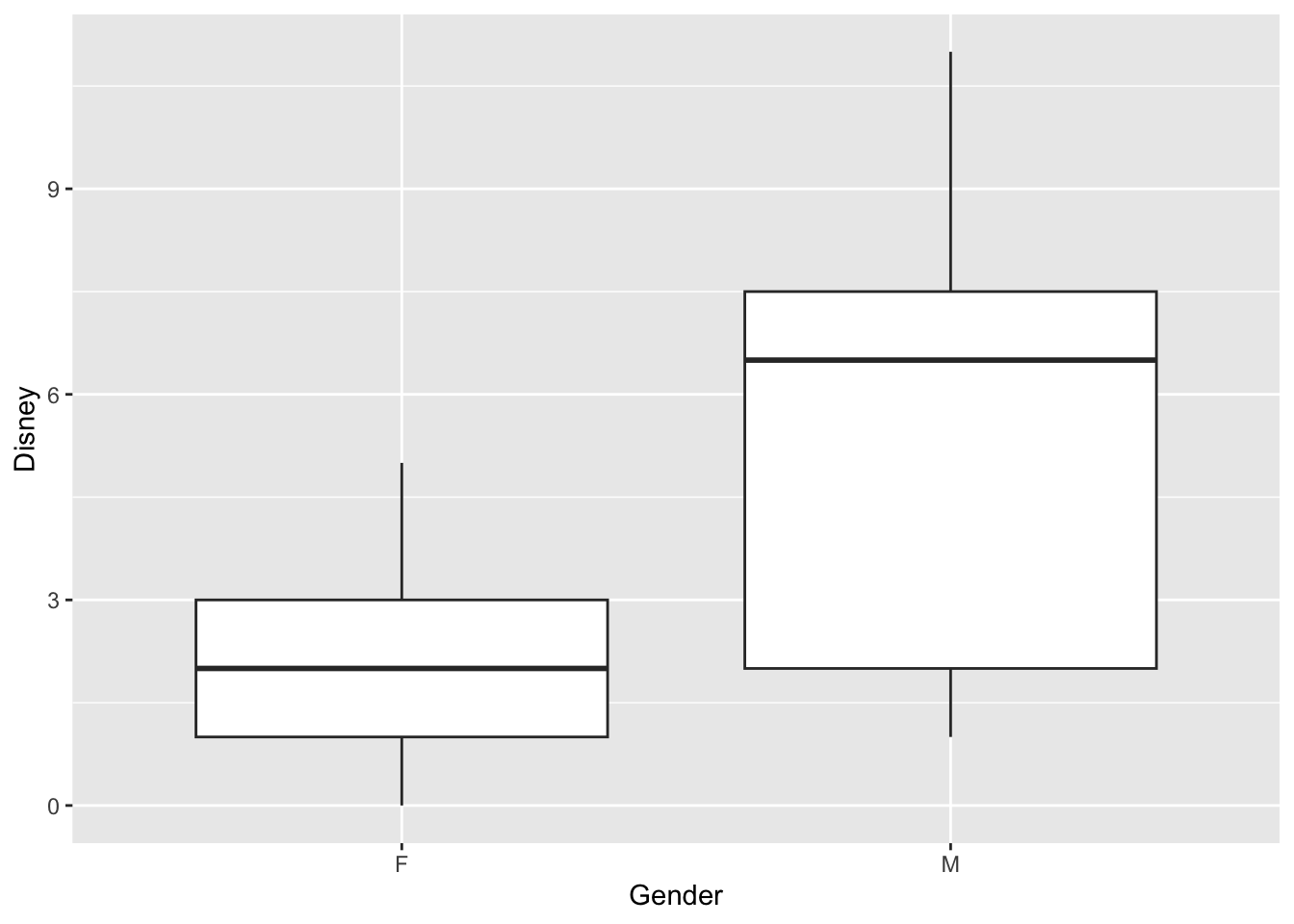
How many time have you gone to Disney, and is there a difference between genders?

Use Wilcoxon Test

Disney=c(3,5,0,1,2,
         0,2,0,2,3,
         2,1,4, 3, 
         2, 1, 2, 6,7,
         11, 7, 9)

Gender=c("F","F","F","F","F",
         "F","F","F","F","F",
         "F","F","F","F",
        "M","M","M","M","M",
        "M","M","M")
DF=data.frame(Disney,Gender)
DF

## Warning in yaml::yaml.load(..., eval.expr = TRUE): NAs introduced by coercion:
## . is not a real

Disney	Gender
3	F
5	F
0	F
1	F
2	F
0	F
2	F
0	F
2	F
3	F
2	F
1	F
4	F
3	F
2	M
1	M
2	M
6	M
7	M
11	M
7	M
9	M

ggplot(DF, aes(y=Disney, x=Gender))+
  geom_boxplot()

ggplot(DF, aes(x=Disney, fill=Gender))+
  geom_histogram()+
  facet_grid(~Gender)

## `stat_bin()` using `bins = 30`.
## Pick better value with
## `binwidth`.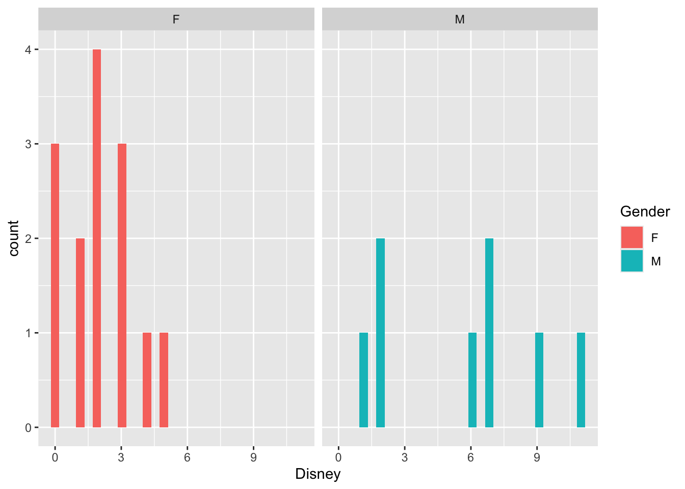

wilcox.test(Disney ~ Gender, data = DF,exact = FALSE, correct= FALSE, conf.int=T )

## 
##  Wilcoxon rank sum test
## 
## data:  Disney by Gender
## W = 24, p-value = 0.02681
## alternative hypothesis: true location shift is not equal to 0
## 95 percent confidence interval:
##  -6.999942e+00 -2.032046e-05
## sample estimates:
## difference in location 
##              -3.999936

Comparing two related conditions: the Wilcoxon signed-rank test (similar to paired t-test)

Do not confuse with the Wilcoxon rank-sum test (similar to unpaired t-test)

We now want to compare the results from sunday and Wendsday, but now the data come from the same individuals. # BDI = Becks depression index Change

drugData$BDIchange<-drugData$wedsBDI-drugData$sundayBDI # calculate differences



drugData$BDIchange

##  [1]  13   0  19   6  20  15   0  13  23  15 -11  -9  10  -7  -7  -6  -8  -2 -15
## [20]  -8

head(drugData)

## Warning in yaml::yaml.load(..., eval.expr = TRUE): NAs introduced by coercion:
## . is not a real

Gender	drug	sundayBDI	wedsBDI	wedsRank	BDIchange
Male	Ecstasy	15	28	12	13
Male	Ecstasy	35	35	17	0
Male	Ecstasy	16	35	17	19
Male	Ecstasy	18	24	10	6
Male	Ecstasy	19	39	20	20
Male	Ecstasy	17	32	15	15

drugData

## Warning in yaml::yaml.load(..., eval.expr = TRUE): NAs introduced by coercion:
## . is not a real

Gender	drug	sundayBDI	wedsBDI	wedsRank	BDIchange
Male	Ecstasy	15	28	12	13
Male	Ecstasy	35	35	17	0
Male	Ecstasy	16	35	17	19
Male	Ecstasy	18	24	10	6
Male	Ecstasy	19	39	20	20
Male	Ecstasy	17	32	15	15
Male	Ecstasy	27	27	11	0
Male	Ecstasy	16	29	13	13
Male	Ecstasy	13	36	19	23
Male	Ecstasy	20	35	17	15
Female	Alcohol	16	5	2	-11
Female	Alcohol	15	6	3.5	-9
Female	Alcohol	20	30	14	10
Female	Alcohol	15	8	6	-7
Female	Alcohol	16	9	7	-7
Female	Alcohol	13	7	5	-6
Female	Alcohol	14	6	3.5	-8
Female	Alcohol	19	17	9	-2
Female	Alcohol	18	3	1	-15
Female	Alcohol	18	10	8	-8

by(drugData$BDIchange, drugData$drug, stat.desc, basic = FALSE, norm = TRUE)

## drugData$drug: Ecstasy
##       median         mean      SE.mean CI.mean.0.95          var      std.dev 
##   14.0000000   12.4000000    2.5307004    5.7248420   64.0444444    8.0027773 
##     coef.var     skewness     skew.2SE     kurtosis     kurt.2SE   normtest.W 
##    0.6453853   -0.4140842   -0.3013525   -1.3686700   -0.5128991    0.9087803 
##   normtest.p 
##    0.2727175 
## ------------------------------------------------------------ 
## drugData$drug: Alcohol
##       median         mean      SE.mean CI.mean.0.95          var      std.dev 
##  -7.50000000  -6.30000000   2.09788253   4.74573999  44.01111111   6.63408706 
##     coef.var     skewness     skew.2SE     kurtosis     kurt.2SE   normtest.W 
##  -1.05302969   1.23907117   0.90174219   0.98664006   0.36973617   0.82795980 
##   normtest.p 
##   0.03161929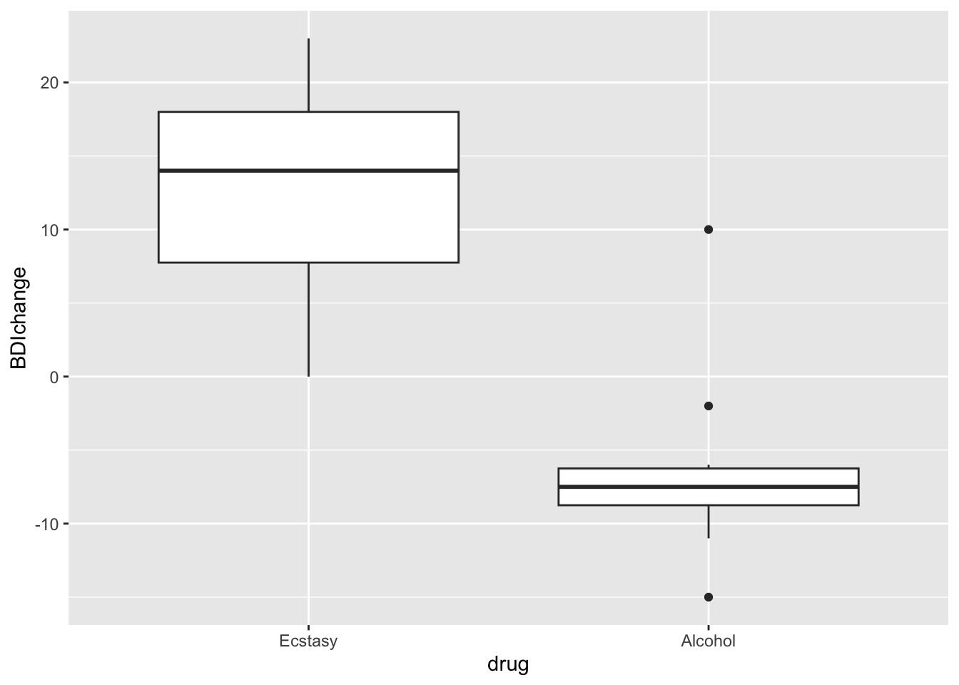

boxplot<-ggplot(drugData, aes(drug, BDIchange)) + 
  geom_boxplot()
boxplot

alcoholData<-subset(drugData, drug == "Alcohol") # subset the data for alcohol
ecstasyData<-subset(drugData, drug == "Ecstasy") # subset the data for ecstasy


alcoholModel<-wilcox.test(alcoholData$wedsBDI, alcoholData$sundayBDI,  paired = TRUE, exact = TRUE, correct= FALSE)

## Warning in wilcox.test.default(alcoholData$wedsBDI, alcoholData$sundayBDI, :
## cannot compute exact p-value with ties

alcoholModel

## 
##  Wilcoxon signed rank test
## 
## data:  alcoholData$wedsBDI and alcoholData$sundayBDI
## V = 8, p-value = 0.04657
## alternative hypothesis: true location shift is not equal to 0

ecstasyModel<-wilcox.test(ecstasyData$wedsBDI, ecstasyData$sundayBDI, paired = TRUE, exact = FALSE,correct= FALSE)   # Note that the option "exact=FALSE" has to be added becase there are ties.  
ecstasyModel

## 
##  Wilcoxon signed rank test
## 
## data:  ecstasyData$wedsBDI and ecstasyData$sundayBDI
## V = 36, p-value = 0.01151
## alternative hypothesis: true location shift is not equal to 0

Krukall-Wallis Test

This is a test similar to ANOVA, thus multiple groups, 3+ grupos

However, you test for the differences in than rank among groups (not the mean).

The null hypothesis is that the sum or mean rank in Ho: G1 = G2 = G3……Gk The alternative hypothesis is that at least one of the groups rank is different from another one.

Soya and the effect on sperm production in human males.

Soy food and isoflavone intake in relation to semen quality parameters among men from an infertility clinic

Jorge E. Chavarro Thomas L. Toth Sonita M. Sadio Russ Hauser Hum Reprod. 2008 Nov;23(11):2584-90. doi: 10.1093/humrep/den243. Epub 2008 Jul 23.

They found that the amount of sperm production is reduced in males which consume more soya

Abstract

BACKGROUND:

High isoflavone intake has been related to decreased fertility in animal studies, but data in humans are scarce. Thus, we examined the association of soy foods and isoflavones intake with semen quality parameters.

METHODS:

The intake of 15 soy-based foods in the previous 3 months was assessed for 99 male partners of subfertile couples who presented for semen analyses to the Massachusetts General Hospital Fertility Center. Linear and quantile regression were used to determine the association of soy foods and isoflavones intake with semen quality parameters while adjusting for personal characteristics.

RESULTS:

There was an inverse association between soy food intake and sperm concentration that remained significant after accounting for age, abstinence time, body mass index, caffeine and alcohol intake and smoking. In the multivariate-adjusted analyses, men in the highest category of soy food intake had 41 million sperm/ml less than men who did not consume soy foods (95% confidence interval = -74, -8; P, trend = 0.02). Results for individual soy isoflavones were similar to the results for soy foods and were strongest for glycitein, but did not reach statistical significance. The inverse relation between soy food intake and sperm concentration was more pronounced in the high end of the distribution (90th and 75th percentile) and among overweight or obese men. Soy food and soy isoflavone intake were unrelated to sperm motility, sperm morphology or ejaculate volume.

CONCLUSIONS:

These data suggest that higher intake of soy foods and soy isoflavones is associated with lower sperm concentration.

Now let us look at the data from Field, soya.csv.

library(readr)

Soyadf <- read_csv("Data_files_csv/Soya.csv")

## Rows: 80 Columns: 2
## ── Column specification ──────────
## Delimiter: ","
## chr (1): Soya
## dbl (1): Sperm
## 
## ℹ Use `spec()` to retrieve the full column specification for this data.
## ℹ Specify the column types or set `show_col_types = FALSE` to quiet this message.

head(Soyadf)

## Warning in yaml::yaml.load(..., eval.expr = TRUE): NAs introduced by coercion:
## . is not a real

Soya	Sperm
No Soya Meals	0.35
No Soya Meals	0.58
No Soya Meals	0.88
No Soya Meals	0.92
No Soya Meals	1.22
No Soya Meals	1.51

unique(Soyadf$Soya)

## [1] "No Soya Meals"          "1 Soya Meal Per Week"   "4 Soyal Meals Per Week"
## [4] "7 Soya Meals Per Week"

Hacer un boxplot de los datos en un nuevo chunk

library(ggplot2)

ggplot(Soyadf, aes(x=Soya, y=Sperm, fill=Soya))+
  geom_boxplot()+
  theme(axis.text.x = element_text(angle = 90))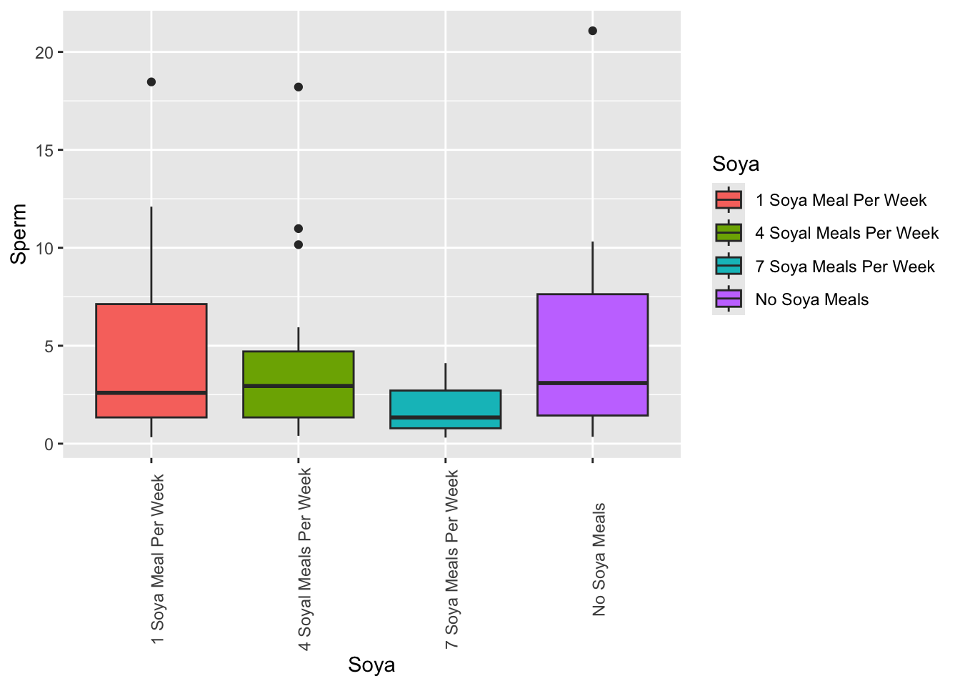

Descriptive statistics When adding “norm=TRUE” will perform Shapiro_Wilks Normality test.

library(pastecs)

by(Soyadf$Sperm, Soyadf$Soya, stat.desc, basic = FALSE, norm = TRUE)

## Soyadf$Soya: 1 Soya Meal Per Week
##       median         mean      SE.mean CI.mean.0.95          var      std.dev 
##  2.595000000  4.606000000  1.044821919  2.186837409 21.833056842  4.672585670 
##     coef.var     skewness     skew.2SE     kurtosis     kurt.2SE   normtest.W 
##  1.014456290  1.350565932  1.318645901  1.422731699  0.716825470  0.825831600 
##   normtest.p 
##  0.002153894 
## ------------------------------------------------------------ 
## Soyadf$Soya: 4 Soyal Meals Per Week
##       median         mean      SE.mean CI.mean.0.95          var      std.dev 
## 2.945000e+00 4.110500e+00 9.861233e-01 2.063980e+00 1.944878e+01 4.410078e+00 
##     coef.var     skewness     skew.2SE     kurtosis     kurt.2SE   normtest.W 
## 1.072881e+00 1.822237e+00 1.779169e+00 2.792615e+00 1.407024e+00 7.427433e-01 
##   normtest.p 
## 1.359072e-04 
## ------------------------------------------------------------ 
## Soyadf$Soya: 7 Soya Meals Per Week
##       median         mean      SE.mean CI.mean.0.95          var      std.dev 
##    1.3350000    1.6535000    0.2479774    0.5190226    1.2298555    1.1089885 
##     coef.var     skewness     skew.2SE     kurtosis     kurt.2SE   normtest.W 
##    0.6706916    0.6086712    0.5942855   -0.9161653   -0.4615984    0.9122606 
##   normtest.p 
##    0.0703908 
## ------------------------------------------------------------ 
## Soyadf$Soya: No Soya Meals
##       median         mean      SE.mean CI.mean.0.95          var      std.dev 
##  3.095000000  4.987000000  1.136926165  2.379613812 25.852022105  5.084488382 
##     coef.var     skewness     skew.2SE     kurtosis     kurt.2SE   normtest.W 
##  1.019548502  1.546140856  1.509598499  2.328051363  1.172959394  0.805255802 
##   normtest.p 
##  0.001035917

Kruskall Wallis test is similar to an ANOVA without assuming normal distribution or equality of variance.

HO: R1=R2=R3=R4 HA: Por lo menos uno los grupos es diferente

# Traditional approach
kruskal.test(Sperm~as.factor(Soya), data=Soyadf)

## 
##  Kruskal-Wallis rank sum test
## 
## data:  Sperm by as.factor(Soya)
## Kruskal-Wallis chi-squared = 8.6589, df = 3, p-value = 0.03419

library(coin)
#Approximative (Monte Carlo) Fisher-Pitman test
modelkt=kruskal_test(Sperm~as.factor(Soya), data=Soyadf, distribution = approximate(nresample = 10000))
modelkt

## 
##  Approximative Kruskal-Wallis Test
## 
## data:  Sperm by
##   as.factor(Soya) (1 Soya Meal Per Week, 4 Soyal Meals Per Week, 7 Soya Meals Per Week, No Soya Meals)
## chi-squared = 8.6589, p-value = 0.0311

#op <- par(no.readonly = TRUE) # save current settings
#layout(matrix(1:3, nrow = 3))
#s1 <- support(modelkt); d1 <- dperm(modelkt, s1)
#plot(s1, d1, type = "h", main = "Mid-score: 0",
#     xlab = "Test Statistic", ylab = "Density")

#pperm(modelkt, q=c(0.05, 0.5, 0.95))


#s=support(modelkt)
#quantile(s, c(.025, 0.975))

Soyadf$Ranks=rank(Soyadf$Sperm)
head(Soyadf)

## Warning in yaml::yaml.load(..., eval.expr = TRUE): NAs introduced by coercion:
## . is not a real

Soya	Sperm	Ranks
No Soya Meals	0.35	4
No Soya Meals	0.58	9
No Soya Meals	0.88	17
No Soya Meals	0.92	18
No Soya Meals	1.22	22
No Soya Meals	1.51	30

by(Soyadf$Ranks, Soyadf$Soya, median)

## Soyadf$Soya: 1 Soya Meal Per Week
## [1] 43
## ------------------------------------------------------------ 
## Soyadf$Soya: 4 Soyal Meals Per Week
## [1] 48.5
## ------------------------------------------------------------ 
## Soyadf$Soya: 7 Soya Meals Per Week
## [1] 25.5
## ------------------------------------------------------------ 
## Soyadf$Soya: No Soya Meals
## [1] 50.5

Post Hoc TUKEY like test (Nemenyi test) The values shown are the p=values, the pair are significantly different if the p is below 0.05

Note

dist=“Tukey”, correction for ties done

library(PMCMRplus)
kwAllPairsNemenyiTest(Sperm~as.factor(Soya) , data=Soyadf)

## 
##  Pairwise comparisons using Tukey-Kramer-Nemenyi all-pairs test with Tukey-Dist approximation

## data: Sperm by as.factor(Soya)

##                        1 Soya Meal Per Week 4 Soyal Meals Per Week
## 4 Soyal Meals Per Week 1.000                -                     
## 7 Soya Meals Per Week  0.101                0.101                 
## No Soya Meals          0.991                0.991                 
##                        7 Soya Meals Per Week
## 4 Soyal Meals Per Week -                    
## 7 Soya Meals Per Week  -                    
## No Soya Meals          0.048

## 
## P value adjustment method: single-step

## alternative hypothesis: two.sided

model1=kwAllPairsNemenyiTest(Sperm~as.factor(Soya) , data=Soyadf) # para más detalles
summary(model1)

## 
##  Pairwise comparisons using Tukey-Kramer-Nemenyi all-pairs test with Tukey-Dist approximation

## data: Sperm by as.factor(Soya)

## alternative hypothesis: two.sided

## P value adjustment method: single-step

## H0

##                                                     q value Pr(>|q|)  
## 4 Soyal Meals Per Week - 1 Soya Meal Per Week == 0    0.000 1.000000  
## 7 Soya Meals Per Week - 1 Soya Meal Per Week == 0     3.233 0.101209  
## No Soya Meals - 1 Soya Meal Per Week == 0             0.423 0.990680  
## 7 Soya Meals Per Week - 4 Soyal Meals Per Week == 0   3.233 0.101209  
## No Soya Meals - 4 Soyal Meals Per Week == 0           0.423 0.990680  
## No Soya Meals - 7 Soya Meals Per Week == 0            3.657 0.047845 *

## ---

## Signif. codes: 0 '***' 0.001 '**' 0.01 '*' 0.05 '.' 0.1 ' ' 1

# Try "Chi Square" = Chisq

15_Non_parametric

RLT

6/26/2017

Los paquetes

Activating packages

Wilcoxon rank-sum test

The hypothesis:

The level of depression posterior to the intake of alcohol is the same as those which take ecstasy.

Is this the null or alternate hipothesis?

Enter raw data

Or Import the data

Exploratory analysis

Descriptive statistics.

Do a histogram by factor level for anxiety for Sunday.

Test of equality of variance

Wilcoxon rank-sum test

This is how to assing the Rank by Hand…… This is an example, the scripts will do this automatically.

Wilcoxon test: A non-parametric test

the following approach is better because it can deal with ties (values that are equal)

Class Excercise

How many time have you gone to Disney, and is there a difference between genders?

Krukall-Wallis Test

Soya and the effect on sperm production in human males.

Soy food and isoflavone intake in relation to semen quality parameters among men from an infertility clinic

Abstract

BACKGROUND:

METHODS:

RESULTS:

CONCLUSIONS:

Hacer un boxplot de los datos en un nuevo chunk

Kruskall Wallis test is similar to an ANOVA without assuming normal distribution or equality of variance.

Note