Usage
ge_cluster(
  .data,
  env = NULL,
  gen = NULL,
  resp = NULL,
  table = FALSE,
  distmethod = "euclidean",
  clustmethod = "ward.D",
  scale = TRUE,
  cluster = "env",
  nclust = NULL
)
Arguments
- .data
The dataset containing the columns related to Environments, Genotypes and the response variable. It is also possible to use a two-way table with genotypes in lines and environments in columns as input. In this case you must use
table = TRUE.- env
The name of the column that contains the levels of the environments. Defaults to
NULL, in case of the input data is a two-way table.- gen
The name of the column that contains the levels of the genotypes. Defaults to
NULL, in case of the input data is a two-way table.- resp
The response variable(s). Defaults to
NULL, in case of the input data is a two-way table.- table
Logical values indicating if the input data is a two-way table with genotypes in the rows and environments in the columns. Defaults to
FALSE.- distmethod
The distance measure to be used. This must be one of
'euclidean','maximum','manhattan','canberra','binary', or'minkowski'.- clustmethod
The agglomeration method to be used. This should be one of
'ward.D'(Default),'ward.D2','single','complete','average'(= UPGMA),'mcquitty'(= WPGMA),'median'(= WPGMC) or'centroid'(= UPGMC).- scale
Should the data be scaled befor computing the distances? Set to TRUE. Let \(Y_{ij}\) be the yield of Hybrid i in Location j, \(\bar Y_{.j}\) be the mean yield, and \(S_j\) be the standard deviation of Location j. The standardized yield (Zij) is computed as (Ouyang et al. 1995): \(Z_{ij} = (Y_{ij} - Y_{.j}) / S_j\).
- cluster
What should be clustered? Defaults to
cluster = "env"(cluster environments). To cluster the genotypes usecluster = "gen".- nclust
The number of clust to be formed. Set to
NULL.
Value
data The data that was used to compute the distances.
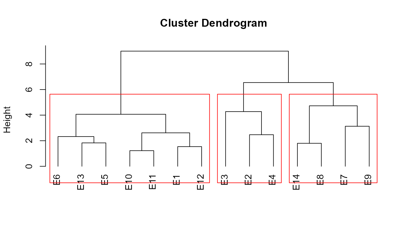
cutpoint The cutpoint of the dendrogram according to Mojena (1977).
distance The matrix with the distances.
de The distances in an object of class
dist.hc The hierarchical clustering.
cophenetic The cophenetic correlation coefficient between distance matrix and cophenetic matrix
Sqt The total sum of squares.
tab A table with the clusters and similarity.
clusters The sum of square and the mean of the clusters for each genotype (if
cluster = "env"or environment (ifcluster = "gen").labclust The labels of genotypes/environments within each cluster.
References
Mojena, R. 2015. Hierarchical grouping methods and stopping rules: an evaluation. Comput. J. 20:359-363. doi:10.1093/comjnl/20.4.359
Ouyang, Z., R.P. Mowers, A. Jensen, S. Wang, and S. Zheng. 1995. Cluster analysis for genotype x environment interaction with unbalanced data. Crop Sci. 35:1300-1305. doi:10.2135/cropsci1995.0011183X003500050008x
Author
Tiago Olivoto tiagoolivoto@gmail.com

