Graphs of the Canonical Correlation Analysis
Usage
# S3 method for can_cor
plot(
  x,
  type = 1,
  plot_theme = theme_metan(),
  size.tex.lab = 12,
  size.tex.pa = 3.5,
  x.lab = NULL,
  x.lim = NULL,
  x.breaks = waiver(),
  y.lab = NULL,
  y.lim = NULL,
  y.breaks = waiver(),
  axis.expand = 1.1,
  shape = 21,
  col.shape = "orange",
  col.alpha = 0.9,
  size.shape = 3.5,
  size.bor.tick = 0.3,
  labels = FALSE,
  main = NULL,
  ...
)
Arguments
- x
The
waasb object- type
The type of the plot. Defaults to
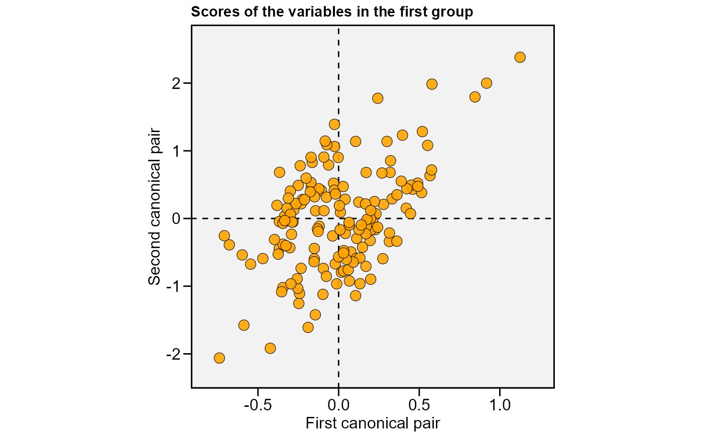
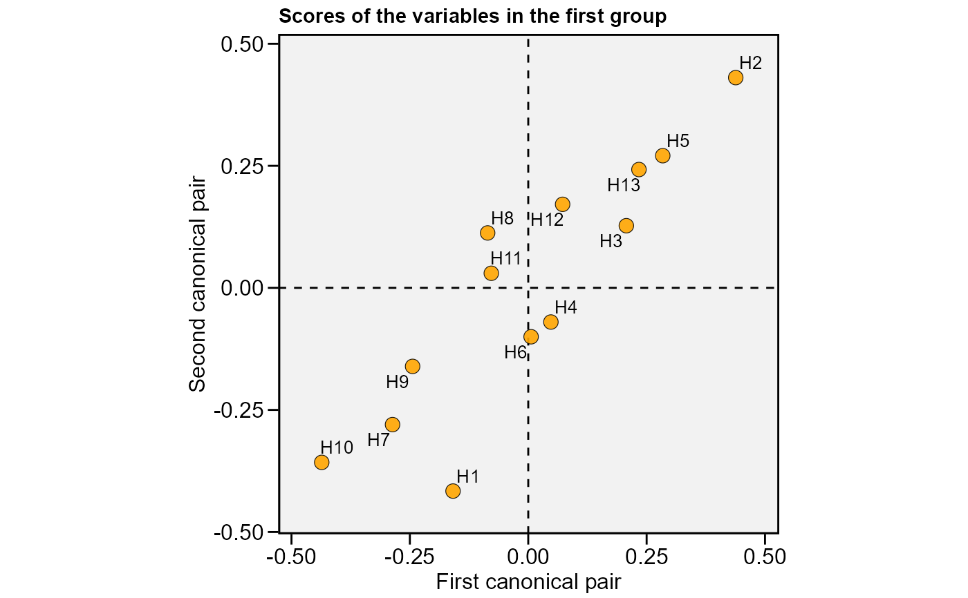
type = 1(Scree-plot of the correlations of the canonical loadings). Usetype = 2, to produce a plot with the scores of the variables in the first group,type = 3to produce a plot with the scores of the variables in the second group, ortype = 4to produce a circle of correlations.- plot_theme
The graphical theme of the plot. Default is
plot_theme = theme_metan(). For more details,seeggplot2::theme().- size.tex.lab
The size of the text in axis text and labels.
- size.tex.pa
The size of the text of the plot area. Default is
3.5.- x.lab
The label of x-axis. Each plot has a default value. New arguments can be inserted as
x.lab = 'my label'.- x.lim
The range of x-axis. Default is
NULL(maximum and minimum values of the data set). New arguments can be inserted asx.lim = c(x.min, x.max).- x.breaks
The breaks to be plotted in the x-axis. Default is
authomatic breaks. New arguments can be inserted asx.breaks = c(breaks)- y.lab
The label of y-axis. Each plot has a default value. New arguments can be inserted as
y.lab = 'my label'.- y.lim
The range of y-axis. Default is
NULL. The same arguments thanx.limcan be used.- y.breaks
The breaks to be plotted in the x-axis. Default is
authomatic breaks. The same arguments thanx.breakscan be used.- axis.expand
Multiplication factor to expand the axis limits by to enable fitting of labels. Default is
1.1.- shape
The shape of points in the plot. Default is
21(circle). Values must be between21-25:21(circle),22(square),23(diamond),24(up triangle), and25(low triangle).- col.shape
A vector of length 2 that contains the color of shapes for genotypes above and below of the mean, respectively. Defaults to
"orange".c("blue", "red").- col.alpha
The alpha value for the color. Default is
0.9. Values must be between0(full transparency) to1(full color).- size.shape
The size of the shape in the plot. Default is
3.5.- size.bor.tick
The size of tick of shape. Default is
0.3. The size of the shape will besize.shape + size.bor.tick- labels
Logical arguments. If
TRUEthen the points in the plot will have labels.- main
The title of the plot. Defaults to
NULL, in which each plot will have a default title. Use a string text to create an own title or set tomain = FALSEto omit the plot title.- ...
Currently not used.
Author
Tiago Olivoto tiagoolivoto@gmail.com
Examples
# \donttest{
library(metan)
cc1 = can_corr(data_ge2,
FG = c(PH, EH, EP),
SG = c(EL, ED, CL, CD, CW, KW, NR))
#> ---------------------------------------------------------------------------
#> Matrix (correlation/covariance) between variables of first group (FG)
#> ---------------------------------------------------------------------------
#> PH EH EP
#> PH 1.0000000 0.9318282 0.6384123
#> EH 0.9318282 1.0000000 0.8695460
#> EP 0.6384123 0.8695460 1.0000000
#> ---------------------------------------------------------------------------
#> Collinearity within first group
#> ---------------------------------------------------------------------------
#> The multicollinearity in the matrix should be investigated.
#> CN = 977.586
#> Largest VIF = 229.164618380199
#> Matrix determinant: 0.0025852
#> Largest correlation: PH x EH = 0.932
#> Smallest correlation: PH x EP = 0.638
#> Number of VIFs > 10: 3
#> Number of correlations with r >= |0.8|: 2
#> Variables with largest weight in the last eigenvalues:
#> EH > PH > EP
#> ---------------------------------------------------------------------------
#> Matrix (correlation/covariance) between variables of second group (SG)
#> ---------------------------------------------------------------------------
#> EL ED CL CD CW KW NR
#> EL 1.00000000 0.3851451 0.2554068 0.91186526 0.4581728 0.6685601 -0.01387378
#> ED 0.38514512 1.0000000 0.6974629 0.38971282 0.7371305 0.8241426 0.55253448
#> CL 0.25540676 0.6974629 1.0000000 0.30036364 0.7383379 0.4709310 0.26193592
#> CD 0.91186526 0.3897128 0.3003636 1.00000000 0.4840299 0.6259806 -0.03584984
#> CW 0.45817278 0.7371305 0.7383379 0.48402989 1.0000000 0.7348622 0.16565752
#> KW 0.66856012 0.8241426 0.4709310 0.62598062 0.7348622 1.0000000 0.36214470
#> NR -0.01387378 0.5525345 0.2619359 -0.03584984 0.1656575 0.3621447 1.00000000
#> ---------------------------------------------------------------------------
#> Collinearity within second group
#> ---------------------------------------------------------------------------
#> Weak multicollinearity in the matrix
#> CN = 68.376
#> Matrix determinant: 0.0015322
#> Largest correlation: EL x CD = 0.912
#> Smallest correlation: EL x NR = -0.014
#> Number of VIFs > 10: 0
#> Number of correlations with r >= |0.8|: 2
#> Variables with largest weight in the last eigenvalues:
#> KW > ED > EL > CD > CL > CW > NR
#> ---------------------------------------------------------------------------
#> Matrix (correlation/covariance) between FG and SG
#> ---------------------------------------------------------------------------
#> EL ED CL CD CW KW NR
#> PH 0.3801960 0.6613148 0.3251648 0.3153910 0.5047388 0.7534439 0.3286065
#> EH 0.3626537 0.6302561 0.3971935 0.2805118 0.5193136 0.7029469 0.2648051
#> EP 0.2634237 0.4580196 0.3908239 0.1750448 0.4248098 0.4974193 0.1404315
#> ---------------------------------------------------------------------------
#> Correlation of the canonical pairs and hypothesis testing
#> ---------------------------------------------------------------------------
#> Var Percent Sum Corr Lambda Chisq DF p_val
#> U1V1 0.6315391 76.189861 76.18986 0.7946943 0.29647 181.76246 21 0.00000
#> U2V2 0.1867300 22.527394 98.71725 0.4321226 0.80462 32.49857 12 0.00116
#> U3V3 0.0106327 1.282745 100.00000 0.1031150 0.98937 1.59810 5 0.90148
#> ---------------------------------------------------------------------------
#> Canonical coefficients of the first group
#> ---------------------------------------------------------------------------
#> U1 U2 U3
#> PH 2.526492 5.866685 7.317151
#> EH -2.436372 -8.263008 -12.447948
#> EP 1.144533 2.747079 6.487414
#> ---------------------------------------------------------------------------
#> Canonical coefficients of the second group
#> ---------------------------------------------------------------------------
#> V1 V2 V3
#> EL -0.00892526 -0.9360837 0.7670684
#> ED 0.19371881 0.2969851 -1.8240876
#> CL -0.08385387 -1.2150642 0.1719827
#> CD -0.30662013 1.1369520 -1.4230311
#> CW -0.15225785 0.1913916 0.4777071
#> KW 1.16752245 -0.1255657 1.1247216
#> NR -0.05865868 0.4861885 0.6223953
#> ---------------------------------------------------------------------------
#> Canonical loads of the first group
#> ---------------------------------------------------------------------------
#> U1 U2 U3
#> PH 0.9868962 -0.07924975 -0.14055369
#> EH 0.9131089 -0.40755395 0.01148369
#> EP 0.6389394 -0.69262240 0.33470980
#> ---------------------------------------------------------------------------
#> Canonical loads of the second group
#> ---------------------------------------------------------------------------
#> V1 V2 V3
#> EL 0.4762839 -0.09829294 -0.22697572
#> ED 0.8298627 -0.16168789 -0.34031848
#> CL 0.3789207 -0.69598199 -0.28635983
#> CD 0.3948013 0.03075542 -0.46981539
#> CW 0.6243739 -0.37712156 -0.14762207
#> KW 0.9566482 -0.05042023 -0.09910729
#> NR 0.4351188 0.29047403 0.18639351
plot(cc1, 2)
 cc2 <-
data_ge2 %>%
mean_by(GEN) %>%
column_to_rownames("GEN") %>%
can_corr(FG = c(PH, EH, EP),
SG = c(EL, ED, CL, CD, CW, KW, NR))
#> ---------------------------------------------------------------------------
#> Matrix (correlation/covariance) between variables of first group (FG)
#> ---------------------------------------------------------------------------
#> PH EH EP
#> PH 1.0000000 0.9189173 0.3939778
#> EH 0.9189173 1.0000000 0.7192828
#> EP 0.3939778 0.7192828 1.0000000
#> ---------------------------------------------------------------------------
#> Collinearity within first group
#> ---------------------------------------------------------------------------
#> The multicollinearity in the matrix should be investigated.
#> CN = 919.528
#> Largest VIF = 221.547716810886
#> Matrix determinant: 0.0038131
#> Largest correlation: PH x EH = 0.919
#> Smallest correlation: PH x EP = 0.394
#> Number of VIFs > 10: 3
#> Number of correlations with r >= |0.8|: 1
#> Variables with largest weight in the last eigenvalues:
#> EH > PH > EP
#> ---------------------------------------------------------------------------
#> Matrix (correlation/covariance) between variables of second group (SG)
#> ---------------------------------------------------------------------------
#> EL ED CL CD CW KW NR
#> EL 1.00000000 0.4010411 0.5131577 0.9377211 0.6957997 0.6563793 -0.07225443
#> ED 0.40104108 1.0000000 0.8486848 0.3152407 0.7881641 0.8950824 0.69413451
#> CL 0.51315772 0.8486848 1.0000000 0.4256584 0.8716229 0.7125578 0.58994313
#> CD 0.93772107 0.3152407 0.4256584 1.0000000 0.6238673 0.5902949 -0.18145262
#> CW 0.69579970 0.7881641 0.8716229 0.6238673 1.0000000 0.8535102 0.50440841
#> KW 0.65637931 0.8950824 0.7125578 0.5902949 0.8535102 1.0000000 0.46907822
#> NR -0.07225443 0.6941345 0.5899431 -0.1814526 0.5044084 0.4690782 1.00000000
#> ---------------------------------------------------------------------------
#> Collinearity within second group
#> ---------------------------------------------------------------------------
#> Severe multicollinearity in the matrix! Pay attention on the variables listed bellow
#> CN = 1552.123
#> Matrix determinant: 7.9e-06
#> Largest correlation: EL x CD = 0.938
#> Smallest correlation: EL x NR = -0.072
#> Number of VIFs > 10: 6
#> Number of correlations with r >= |0.8|: 5
#> Variables with largest weight in the last eigenvalues:
#> ED > KW > CL > CW > EL > NR > CD
#> ---------------------------------------------------------------------------
#> Matrix (correlation/covariance) between FG and SG
#> ---------------------------------------------------------------------------
#> EL ED CL CD CW KW NR
#> PH 0.2290182 0.7918292 0.5262760 0.2345645 0.6530199 0.8224189 0.45295974
#> EH 0.3025919 0.7768116 0.6219269 0.2729626 0.6736994 0.7936528 0.33082529
#> EP 0.3682229 0.4971223 0.5993264 0.2888874 0.4874277 0.4732954 0.04794453
#> ---------------------------------------------------------------------------
#> Correlation of the canonical pairs and hypothesis testing
#> ---------------------------------------------------------------------------
#> Var Percent Sum Corr Lambda Chisq DF p_val
#> U1V1 0.9718658 41.47197 41.47197 0.9858325 0.00218 39.83935 21 0.00778
#> U2V2 0.8317335 35.49217 76.96414 0.9119942 0.07743 16.62936 12 0.16408
#> U3V3 0.5398289 23.03586 100.00000 0.7347305 0.46017 5.04502 5 0.41041
#> ---------------------------------------------------------------------------
#> Canonical coefficients of the first group
#> ---------------------------------------------------------------------------
#> U1 U2 U3
#> PH 5.773517 6.359457 7.266106
#> EH -6.410034 -8.561079 -10.352155
#> EP 2.560042 2.837721 5.118397
#> ---------------------------------------------------------------------------
#> Canonical coefficients of the second group
#> ---------------------------------------------------------------------------
#> V1 V2 V3
#> EL -0.59514582 0.8165268 0.7660462
#> ED 2.24335840 4.5202765 -1.7746076
#> CL -1.60643643 -3.6532159 2.6019702
#> CD 0.81059969 1.4810578 0.1877906
#> CW 1.11115714 1.4920125 -2.5251980
#> KW -1.03618614 -4.8770282 1.2249614
#> NR 0.04635339 1.0825779 0.6376536
#> ---------------------------------------------------------------------------
#> Canonical loads of the first group
#> ---------------------------------------------------------------------------
#> U1 U2 U3
#> PH 0.8918261 -0.3894677 -0.230132932
#> EH 0.7367446 -0.6761412 0.006369758
#> EP 0.2240527 -0.8146310 0.534954830
#> ---------------------------------------------------------------------------
#> Canonical loads of the second group
#> ---------------------------------------------------------------------------
#> V1 V2 V3
#> EL 0.3299566 -0.09777307 0.5666060
#> ED 0.8773340 -0.22373844 0.3488486
#> CL 0.5946161 -0.30352692 0.6169395
#> CD 0.3490720 -0.02781792 0.4862462
#> CW 0.7096748 -0.25390402 0.3613829
#> KW 0.8851044 -0.24266216 0.2480914
#> NR 0.6261809 0.20220468 0.1522980
plot(cc2, 2, labels = TRUE)
cc2 <-
data_ge2 %>%
mean_by(GEN) %>%
column_to_rownames("GEN") %>%
can_corr(FG = c(PH, EH, EP),
SG = c(EL, ED, CL, CD, CW, KW, NR))
#> ---------------------------------------------------------------------------
#> Matrix (correlation/covariance) between variables of first group (FG)
#> ---------------------------------------------------------------------------
#> PH EH EP
#> PH 1.0000000 0.9189173 0.3939778
#> EH 0.9189173 1.0000000 0.7192828
#> EP 0.3939778 0.7192828 1.0000000
#> ---------------------------------------------------------------------------
#> Collinearity within first group
#> ---------------------------------------------------------------------------
#> The multicollinearity in the matrix should be investigated.
#> CN = 919.528
#> Largest VIF = 221.547716810886
#> Matrix determinant: 0.0038131
#> Largest correlation: PH x EH = 0.919
#> Smallest correlation: PH x EP = 0.394
#> Number of VIFs > 10: 3
#> Number of correlations with r >= |0.8|: 1
#> Variables with largest weight in the last eigenvalues:
#> EH > PH > EP
#> ---------------------------------------------------------------------------
#> Matrix (correlation/covariance) between variables of second group (SG)
#> ---------------------------------------------------------------------------
#> EL ED CL CD CW KW NR
#> EL 1.00000000 0.4010411 0.5131577 0.9377211 0.6957997 0.6563793 -0.07225443
#> ED 0.40104108 1.0000000 0.8486848 0.3152407 0.7881641 0.8950824 0.69413451
#> CL 0.51315772 0.8486848 1.0000000 0.4256584 0.8716229 0.7125578 0.58994313
#> CD 0.93772107 0.3152407 0.4256584 1.0000000 0.6238673 0.5902949 -0.18145262
#> CW 0.69579970 0.7881641 0.8716229 0.6238673 1.0000000 0.8535102 0.50440841
#> KW 0.65637931 0.8950824 0.7125578 0.5902949 0.8535102 1.0000000 0.46907822
#> NR -0.07225443 0.6941345 0.5899431 -0.1814526 0.5044084 0.4690782 1.00000000
#> ---------------------------------------------------------------------------
#> Collinearity within second group
#> ---------------------------------------------------------------------------
#> Severe multicollinearity in the matrix! Pay attention on the variables listed bellow
#> CN = 1552.123
#> Matrix determinant: 7.9e-06
#> Largest correlation: EL x CD = 0.938
#> Smallest correlation: EL x NR = -0.072
#> Number of VIFs > 10: 6
#> Number of correlations with r >= |0.8|: 5
#> Variables with largest weight in the last eigenvalues:
#> ED > KW > CL > CW > EL > NR > CD
#> ---------------------------------------------------------------------------
#> Matrix (correlation/covariance) between FG and SG
#> ---------------------------------------------------------------------------
#> EL ED CL CD CW KW NR
#> PH 0.2290182 0.7918292 0.5262760 0.2345645 0.6530199 0.8224189 0.45295974
#> EH 0.3025919 0.7768116 0.6219269 0.2729626 0.6736994 0.7936528 0.33082529
#> EP 0.3682229 0.4971223 0.5993264 0.2888874 0.4874277 0.4732954 0.04794453
#> ---------------------------------------------------------------------------
#> Correlation of the canonical pairs and hypothesis testing
#> ---------------------------------------------------------------------------
#> Var Percent Sum Corr Lambda Chisq DF p_val
#> U1V1 0.9718658 41.47197 41.47197 0.9858325 0.00218 39.83935 21 0.00778
#> U2V2 0.8317335 35.49217 76.96414 0.9119942 0.07743 16.62936 12 0.16408
#> U3V3 0.5398289 23.03586 100.00000 0.7347305 0.46017 5.04502 5 0.41041
#> ---------------------------------------------------------------------------
#> Canonical coefficients of the first group
#> ---------------------------------------------------------------------------
#> U1 U2 U3
#> PH 5.773517 6.359457 7.266106
#> EH -6.410034 -8.561079 -10.352155
#> EP 2.560042 2.837721 5.118397
#> ---------------------------------------------------------------------------
#> Canonical coefficients of the second group
#> ---------------------------------------------------------------------------
#> V1 V2 V3
#> EL -0.59514582 0.8165268 0.7660462
#> ED 2.24335840 4.5202765 -1.7746076
#> CL -1.60643643 -3.6532159 2.6019702
#> CD 0.81059969 1.4810578 0.1877906
#> CW 1.11115714 1.4920125 -2.5251980
#> KW -1.03618614 -4.8770282 1.2249614
#> NR 0.04635339 1.0825779 0.6376536
#> ---------------------------------------------------------------------------
#> Canonical loads of the first group
#> ---------------------------------------------------------------------------
#> U1 U2 U3
#> PH 0.8918261 -0.3894677 -0.230132932
#> EH 0.7367446 -0.6761412 0.006369758
#> EP 0.2240527 -0.8146310 0.534954830
#> ---------------------------------------------------------------------------
#> Canonical loads of the second group
#> ---------------------------------------------------------------------------
#> V1 V2 V3
#> EL 0.3299566 -0.09777307 0.5666060
#> ED 0.8773340 -0.22373844 0.3488486
#> CL 0.5946161 -0.30352692 0.6169395
#> CD 0.3490720 -0.02781792 0.4862462
#> CW 0.7096748 -0.25390402 0.3613829
#> KW 0.8851044 -0.24266216 0.2480914
#> NR 0.6261809 0.20220468 0.1522980
plot(cc2, 2, labels = TRUE)
 # }
# }