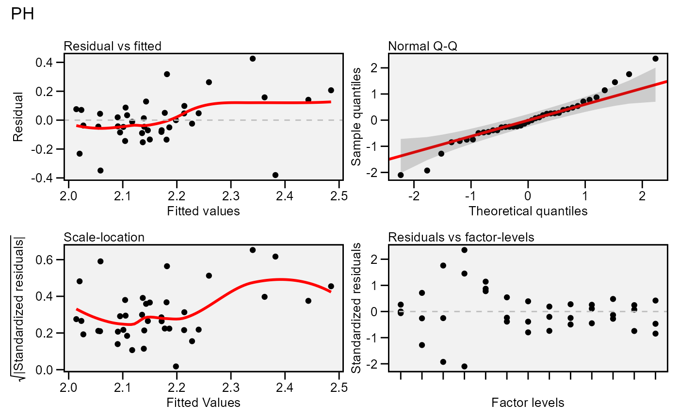
Several types of residual plots — plot.gamem • metan

Residual plots for a output model of class gamem. Six types of plots are produced: (1) Residuals vs fitted, (2) normal Q-Q plot for the residuals, (3) scale-location plot (standardized residuals vs Fitted Values), (4) standardized residuals vs Factor-levels, (5) Histogram of raw residuals and (6) standardized residuals vs observation order. For a waasb object, normal Q-Q plot for random effects may also be obtained declaring type = 're'

Usage

# S3 method for gamem
plot(
  x,
  var = 1,
  type = "res",
  position = "fill",
  rotate = FALSE,
  conf = 0.95,
  out = "print",
  n.dodge = 1,
  check.overlap = FALSE,
  labels = FALSE,
  plot_theme = theme_metan(),
  alpha = 0.2,
  fill.hist = "gray",
  col.hist = "black",
  col.point = "black",
  col.line = "red",
  col.lab.out = "red",
  size.line = 0.7,
  size.text = 10,
  width.bar = 0.75,
  size.lab.out = 2.5,
  size.tex.lab = 10,
  size.shape = 1.5,
  bins = 30,
  which = c(1:4),
  ncol = NULL,
  nrow = NULL,
  ...
)

Arguments

x: An object of class gamem.
var: The variable to plot. Defaults to var = 1 the first variable of x.
type: One of the "res" to plot the model residuals (default), type = 're' to plot normal Q-Q plots for the random effects, or "vcomp" to create a bar plot with the variance components.
position: The position adjustment when type = "vcomp". Defaults to "fill", which shows relative proportions at each trait by stacking the bars and then standardizing each bar to have the same height. Use position = "stack" to plot the phenotypic variance for each trait.
rotate: Logical argument. If rotate = TRUE the plot is rotated, i.e., traits in y axis and value in the x axis.
conf: Level of confidence interval to use in the Q-Q plot (0.95 by default).
out: How the output is returned. Must be one of the 'print' (default) or 'return'.
n.dodge: The number of rows that should be used to render the x labels. This is useful for displaying labels that would otherwise overlap.
check.overlap: Silently remove overlapping labels, (recursively) prioritizing the first, last, and middle labels.
labels: Logical argument. If TRUE labels the points outside confidence interval limits.
plot_theme: The graphical theme of the plot. Default is plot_theme = theme_metan(). For more details, see ggplot2::theme().
alpha: The transparency of confidence band in the Q-Q plot. Must be a number between 0 (opaque) and 1 (full transparency).
fill.hist: The color to fill the histogram. Default is 'gray'.
col.hist: The color of the border of the the histogram. Default is 'black'.
col.point: The color of the points in the graphic. Default is 'black'.
col.line: The color of the lines in the graphic. Default is 'red'.
col.lab.out: The color of the labels for the 'outlying' points.
size.line: The size of the line in graphic. Defaults to 0.7.
size.text: The size for the text in the plot. Defaults to 10.
width.bar: The width of the bars if type = "contribution".
size.lab.out: The size of the labels for the 'outlying' points.
size.tex.lab: The size of the text in axis text and labels.
size.shape: The size of the shape in the plots.
bins: The number of bins to use in the histogram. Default is 30.
which: Which graphics should be plotted. Default is which = c(1:4) that means that the first four graphics will be plotted.
ncol, nrow: The number of columns and rows of the plot pannel. Defaults to NULL
...: Additional arguments passed on to the function patchwork::wrap_plots().

Author

Tiago Olivoto tiagoolivoto@gmail.com

Examples

# \donttest{
library(metan)
model <- gamem(data_g,
               gen = GEN,
               rep = REP,
               resp = PH)
#> Evaluating trait PH |============================================| 100% 00:00:00 

#> Method: REML/BLUP
#> Random effects: GEN
#> Fixed effects: REP
#> Denominador DF: Satterthwaite's method
#> ---------------------------------------------------------------------------
#> P-values for Likelihood Ratio Test of the analyzed traits
#> ---------------------------------------------------------------------------
#>     model    PH
#>  Complete    NA
#>  Genotype 0.051
#> ---------------------------------------------------------------------------
#> Variables with nonsignificant Genotype effect
#> PH 
#> ---------------------------------------------------------------------------
plot(model)
#> `geom_smooth()` using formula = 'y ~ x'
#> `geom_smooth()` using formula = 'y ~ x'

# }