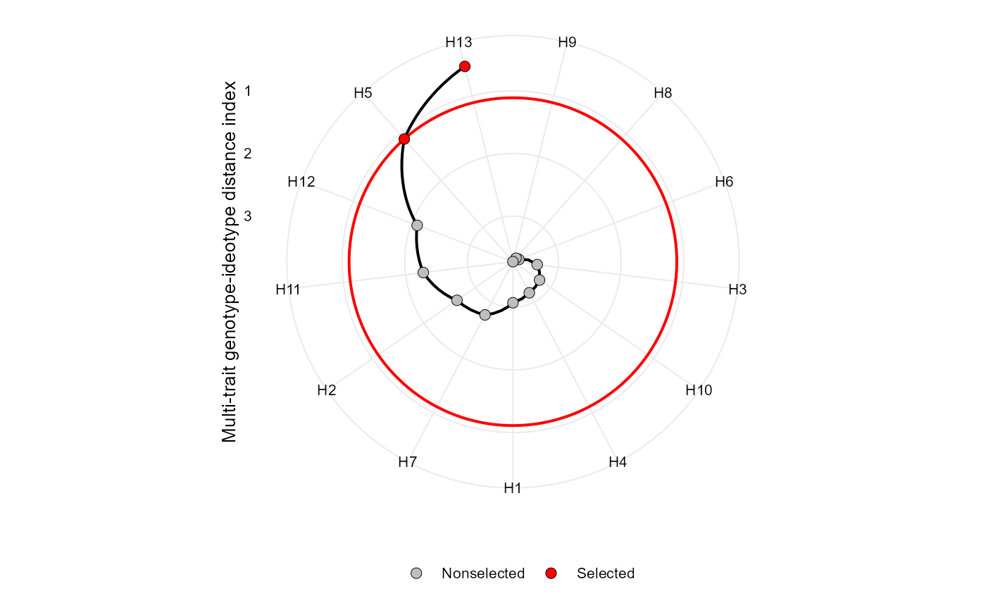
Plot the multi-trait genotype-ideotype distance index

Makes a radar plot showing the multi-trait genotype-ideotype distance index

Usage

# S3 method for mgidi
plot(
  x,
  SI = 15,
  radar = TRUE,
  type = "index",
  position = "fill",
  rotate = FALSE,
  genotypes = "selected",
  n.dodge = 1,
  check.overlap = FALSE,
  x.lab = NULL,
  y.lab = NULL,
  title = NULL,
  arrange.label = FALSE,
  size.point = 2.5,
  size.line = 0.7,
  size.text = 10,
  width.bar = 0.75,
  col.sel = "red",
  col.nonsel = "gray",
  legend.position = "bottom",
  ...
)

Arguments

x: An object of class mgidi
SI: An integer (0-100). The selection intensity in percentage of the total number of genotypes.
radar: Logical argument. If true (default) a radar plot is generated after using coord_polar().
type: The type of the plot. Defaults to "index". Use type = "contribution" to show the contribution of each factor to the MGIDI index of the selected genotypes/treatments.
position: The position adjustment when type = "contribution". Defaults to "fill", which shows relative proportions at each trait by stacking the bars and then standardizing each bar to have the same height. Use position = "stack" to plot the MGIDI index for each genotype/treatment.
rotate: Logical argument. If rotate = TRUE the plot is rotated, i.e., traits in y axis and value in the x axis.
genotypes: When type = "contribution" defines the genotypes to be shown in the plot. By default (genotypes = "selected" only selected genotypes are shown. Use genotypes = "all" to plot the contribution for all genotypes.)
n.dodge: The number of rows that should be used to render the x labels. This is useful for displaying labels that would otherwise overlap.
check.overlap: Silently remove overlapping labels, (recursively) prioritizing the first, last, and middle labels.
x.lab, y.lab: The labels for the axes x and y, respectively. x label is set to null when a radar plot is produced.
title: The plot title when type = "contribution".
arrange.label: Logical argument. If TRUE, the labels are arranged to avoid text overlapping. This becomes useful when the number of genotypes is large, say, more than 30.
size.point: The size of the point in graphic. Defaults to 2.5.
size.line: The size of the line in graphic. Defaults to 0.7.
size.text: The size for the text in the plot. Defaults to 10.
width.bar: The width of the bars if type = "contribution". Defaults to 0.75.
col.sel: The colour for selected genotypes. Defaults to "red".
col.nonsel: The colour for nonselected genotypes. Defaults to "gray".
legend.position: The position of the legend.
...: Other arguments to be passed from ggplot2::theme().

Value

An object of class gg, ggplot.

Author

Tiago Olivoto tiagoolivoto@gmail.com

Examples

# \donttest{
library(metan)
model <- gamem(data_g,
               gen = GEN,
               rep = REP,
               resp = c(KW, NR, NKE, NKR))
#> Evaluating trait KW |===========                                 | 25% 00:00:00 
Evaluating trait NR |======================                      | 50% 00:00:00 
Evaluating trait NKE |================================           | 75% 00:00:00 
Evaluating trait NKR |===========================================| 100% 00:00:00 

#> Method: REML/BLUP
#> Random effects: GEN
#> Fixed effects: REP
#> Denominador DF: Satterthwaite's method
#> ---------------------------------------------------------------------------
#> P-values for Likelihood Ratio Test of the analyzed traits
#> ---------------------------------------------------------------------------
#>     model     KW     NR     NKE   NKR
#>  Complete     NA     NA      NA    NA
#>  Genotype 0.0253 0.0056 0.00952 0.216
#> ---------------------------------------------------------------------------
#> Variables with nonsignificant Genotype effect
#> NKR 
#> ---------------------------------------------------------------------------
mgidi_index <- mgidi(model)
#> 
#> -------------------------------------------------------------------------------
#> Principal Component Analysis
#> -------------------------------------------------------------------------------
#> # A tibble: 4 × 4
#>   PC    Eigenvalues `Variance (%)` `Cum. variance (%)`
#>   <chr>       <dbl>          <dbl>               <dbl>
#> 1 PC1          2.42          60.6                 60.6
#> 2 PC2          1.19          29.8                 90.3
#> 3 PC3          0.32           8                   98.3
#> 4 PC4          0.07           1.66               100  
#> -------------------------------------------------------------------------------
#> Factor Analysis - factorial loadings after rotation-
#> -------------------------------------------------------------------------------
#> # A tibble: 4 × 5
#>   VAR     FA1   FA2 Communality Uniquenesses
#>   <chr> <dbl> <dbl>       <dbl>        <dbl>
#> 1 KW    -0.9   0.04        0.82         0.18
#> 2 NR    -0.92 -0.12        0.87         0.13
#> 3 NKE   -0.7  -0.69        0.96         0.04
#> 4 NKR    0.05 -0.98        0.97         0.03
#> -------------------------------------------------------------------------------
#> Comunalit Mean: 0.9033994 
#> -------------------------------------------------------------------------------
#> Selection differential 
#> -------------------------------------------------------------------------------
#> # A tibble: 4 × 11
#>   VAR   Factor    Xo    Xs     SD SDperc    h2     SG SGperc sense     goal
#>   <chr> <chr>  <dbl> <dbl>  <dbl>  <dbl> <dbl>  <dbl>  <dbl> <chr>    <dbl>
#> 1 KW    FA1    147.  163.  16.2    11.0  0.659 10.7     7.27 increase   100
#> 2 NR    FA1     15.8  17.4  1.63   10.3  0.736  1.20    7.60 increase   100
#> 3 NKE   FA1    468.  532.  64.0    13.7  0.713 45.6     9.74 increase   100
#> 4 NKR   FA2     30.4  31.2  0.814   2.68 0.452  0.368   1.21 increase   100
#> ------------------------------------------------------------------------------
#> Selected genotypes
#> -------------------------------------------------------------------------------
#> H13 H5
#> -------------------------------------------------------------------------------
plot(mgidi_index)

# }