plot sf object

plot one or more attributes of an sf object on a map Plot sf object

# S3 method for sf
plot(
  x,
  y,
  ...,
  main,
  pal = NULL,
  nbreaks = 10,
  breaks = "pretty",
  max.plot = if (is.null(n <- options("sf_max.plot")[[1]])) 9 else n,
  key.pos = get_key_pos(x, ...),
  key.length = 0.618,
  key.width = lcm(1.8),
  reset = TRUE,
  logz = FALSE
)

get_key_pos(x, ...)

# S3 method for sfc_POINT
plot(
  x,
  y,
  ...,
  pch = 1,
  cex = 1,
  col = 1,
  bg = 0,
  lwd = 1,
  lty = 1,
  type = "p",
  add = FALSE
)

# S3 method for sfc_MULTIPOINT
plot(
  x,
  y,
  ...,
  pch = 1,
  cex = 1,
  col = 1,
  bg = 0,
  lwd = 1,
  lty = 1,
  type = "p",
  add = FALSE
)

# S3 method for sfc_LINESTRING
plot(x, y, ..., lty = 1, lwd = 1, col = 1, pch = 1, type = "l", add = FALSE)

# S3 method for sfc_CIRCULARSTRING
plot(x, y, ...)

# S3 method for sfc_MULTILINESTRING
plot(x, y, ..., lty = 1, lwd = 1, col = 1, pch = 1, type = "l", add = FALSE)

# S3 method for sfc_POLYGON
plot(
  x,
  y,
  ...,
  lty = 1,
  lwd = 1,
  col = NA,
  cex = 1,
  pch = NA,
  border = 1,
  add = FALSE,
  rule = "evenodd"
)

# S3 method for sfc_MULTIPOLYGON
plot(
  x,
  y,
  ...,
  lty = 1,
  lwd = 1,
  col = NA,
  border = 1,
  add = FALSE,
  rule = "evenodd"
)

# S3 method for sfc_GEOMETRYCOLLECTION
plot(
  x,
  y,
  ...,
  pch = 1,
  cex = 1,
  bg = 0,
  lty = 1,
  lwd = 1,
  col = 1,
  border = 1,
  add = FALSE
)

# S3 method for sfc_GEOMETRY
plot(
  x,
  y,
  ...,
  pch = 1,
  cex = 1,
  bg = 0,
  lty = 1,
  lwd = 1,
  col = ifelse(st_dimension(x) == 2, NA, 1),
  border = 1,
  add = FALSE
)

# S3 method for sfg
plot(x, ...)

plot_sf(
  x,
  xlim = NULL,
  ylim = NULL,
  asp = NA,
  axes = FALSE,
  bgc = par("bg"),
  ...,
  xaxs,
  yaxs,
  lab,
  setParUsrBB = FALSE,
  bgMap = NULL,
  expandBB = c(0, 0, 0, 0),
  graticule = NA_crs_,
  col_graticule = "grey",
  border
)

sf.colors(n = 10, cutoff.tails = c(0.35, 0.2), alpha = 1, categorical = FALSE)

Arguments

x	object of class sf
y	ignored
...	further specifications, see plot_sf and plot and details.
main	title for plot (NULL to remove)
pal	palette function, similar to rainbow, or palette values; if omitted, sf.colors is used
nbreaks	number of colors breaks (ignored for factor or character variables)
breaks	either a numeric vector with the actual breaks, or a name of a method accepted by the style argument of classIntervals
max.plot	integer; lower boundary to maximum number of attributes to plot; the default value (9) can be overriden by setting the global option sf_max.plot, e.g. options(sf_max.plot=2)
key.pos	integer; side to plot a color key: 1 bottom, 2 left, 3 top, 4 right; set to NULL to omit key, or -1 to select automatically. If multiple columns are plotted in a single function call by default no key is plotted and every submap is stretched individually; if a key is requested (and col is missing) all maps are colored according to a single key. Auto select depends on plot size, map aspect, and, if set, parameter asp.
key.length	amount of space reserved for the key along its axis, length of the scale bar
key.width	amount of space reserved for the key (incl. labels), thickness/width of the scale bar
reset	logical; if FALSE, keep the plot in a mode that allows adding further map elements; if TRUE restore original mode after plotting sf objects with attributes; see details.
logz	logical; if TRUE, use log10-scale for the attribute variable. In that case, breaks and at need to be given as log10-values; see examples.
pch	plotting symbol
cex	symbol size
col	color for plotting features; if length(col) does not equal 1 or nrow(x), a warning is emitted that colors will be recycled. Specifying col suppresses plotting the legend key.
bg	symbol background color
lwd	line width
lty	line type
type	plot type: 'p' for points, 'l' for lines, 'b' for both
add	logical; add to current plot? Note that when using add=TRUE, you may have to set reset=FALSE in the first plot command.
border	color of polygon border(s)
rule	see polypath; for winding, exterior ring direction should be opposite that of the holes; with evenodd, plotting is robust against misspecified ring directions
xlim	see plot.window
ylim	see plot.window
asp	see below, and see par
axes	logical; should axes be plotted? (default FALSE)
bgc	background color
xaxs	see par
yaxs	see par
lab	see par
setParUsrBB	default FALSE; set the par “usr” bounding box; see below
bgMap	object of class ggmap, or returned by function RgoogleMaps::GetMap
expandBB	numeric; fractional values to expand the bounding box with, in each direction (bottom, left, top, right)
graticule	logical, or object of class crs (e.g., st_crs(4326) for a WGS84 graticule), or object created by st_graticule; TRUE will give the WGS84 graticule or object returned by st_graticule
col_graticule	color to used for the graticule (if present)
n	integer; number of colors
cutoff.tails	numeric, in [0,0.5] start and end values
alpha	numeric, in [0,1], transparency
categorical	logical; do we want colors for a categorical variable? (see details)

Details

plot.sf maximally plots max.plot maps with colors following from attribute columns, one map per attribute. It uses sf.colors for default colors. For more control over placement of individual maps, set parameter mfrow with par prior to plotting, and plot single maps one by one; note that this only works in combination with setting parameters key.pos=NULL (no legend) and reset=FALSE.

plot.sfc plots the geometry, additional parameters can be passed on to control color, lines or symbols.

When setting reset to FALSE, the original device parameters are lost, and the device must be reset using dev.off() in order to reset it.

parameter at can be set to specify where labels are placed along the key; see examples.

plot_sf sets up the plotting area, axes, graticule, or webmap background; it is called by all plot methods before anything is drawn.

The argument setParUsrBB may be used to pass the logical value TRUE to functions within plot.Spatial. When set to TRUE, par(“usr”) will be overwritten with c(xlim, ylim), which defaults to the bounding box of the spatial object. This is only needed in the particular context of graphic output to a specified device with given width and height, to be matched to the spatial object, when using par(“xaxs”) and par(“yaxs”) in addition to par(mar=c(0,0,0,0)).

The default aspect for map plots is 1; if however data are not projected (coordinates are long/lat), the aspect is by default set to 1/cos(My * pi/180) with My the y coordinate of the middle of the map (the mean of ylim, which defaults to the y range of bounding box). This implies an Equirectangular projection.

non-categorical colors from sf.colors were taken from bpy.colors, with modified cutoff.tails defaults If categorical is TRUE, default colors are from http://www.colorbrewer2.org/ (if n < 9, Set2, else Set3).

Examples

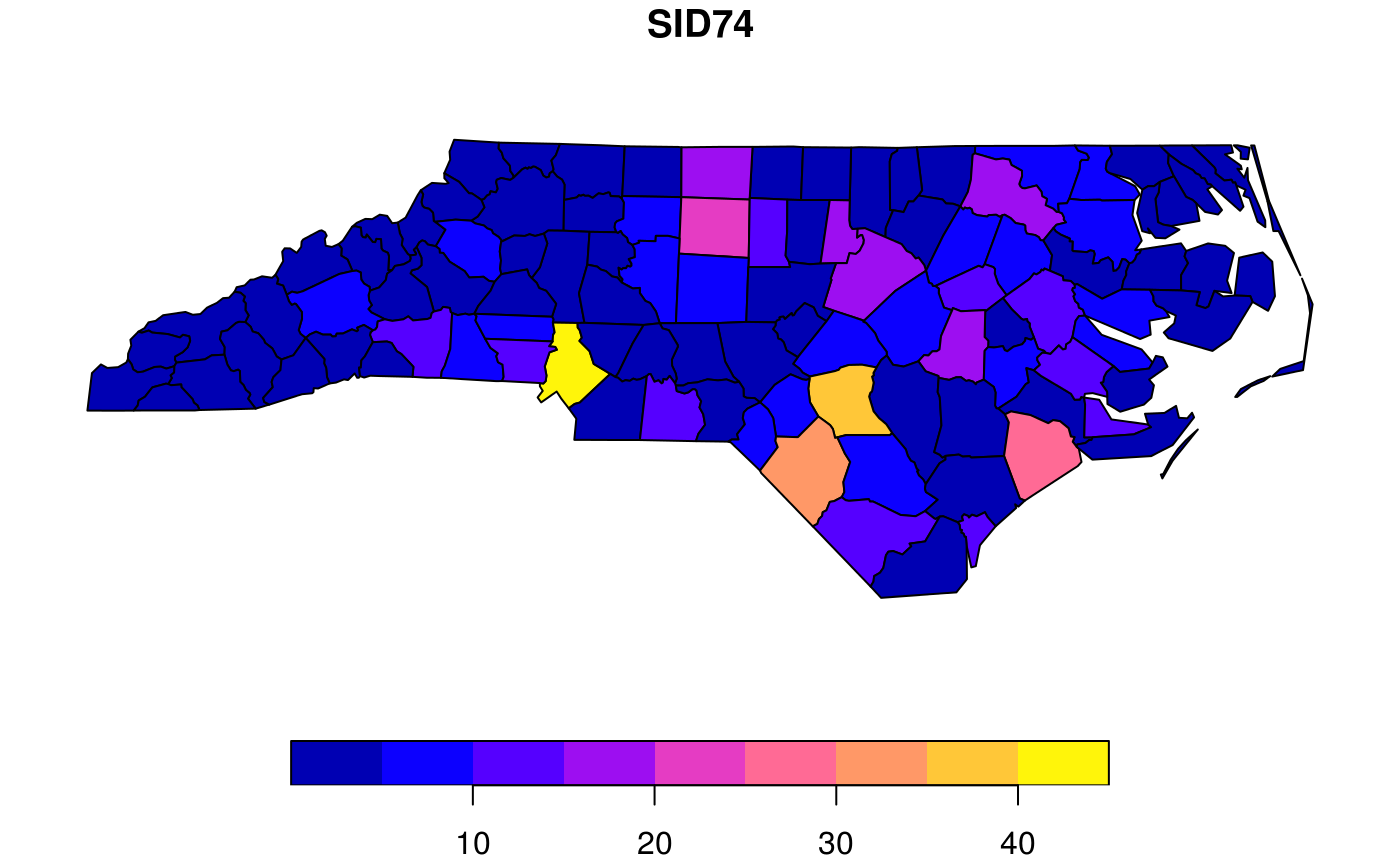
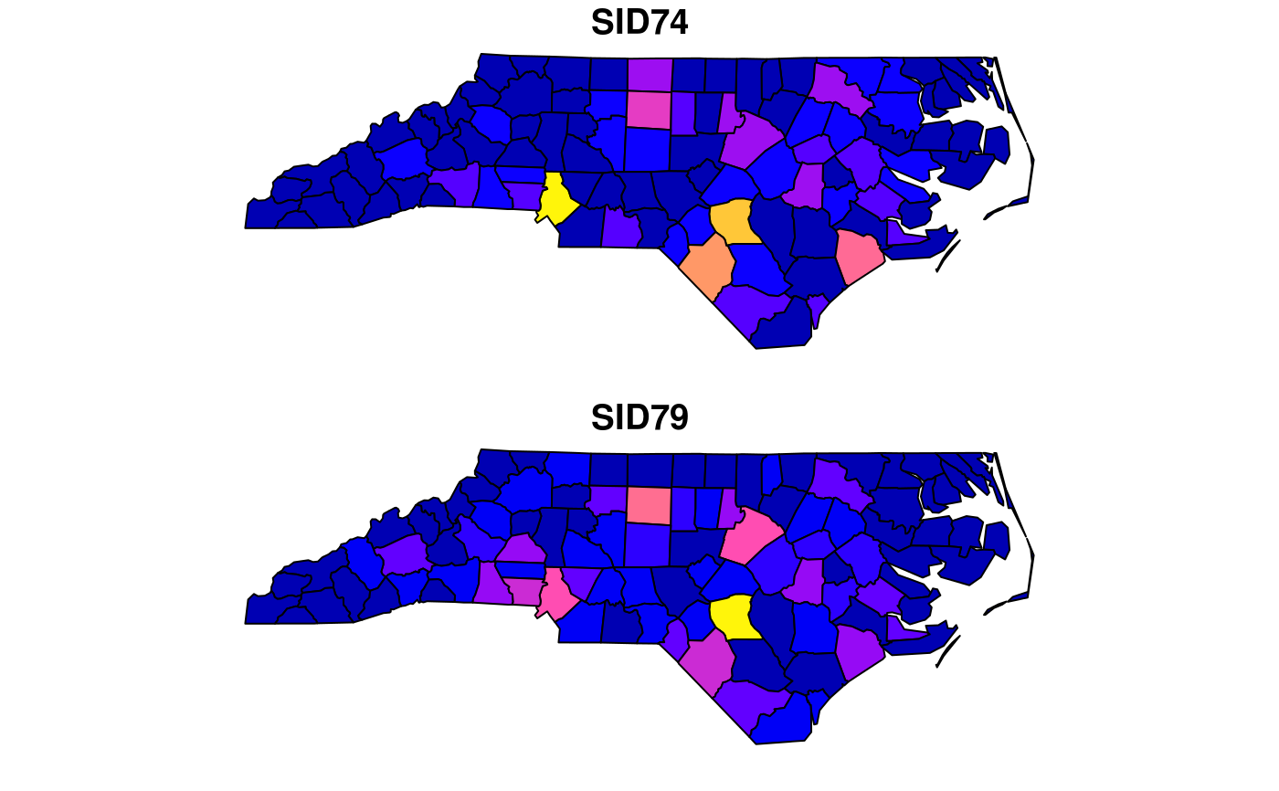
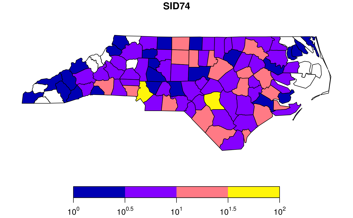
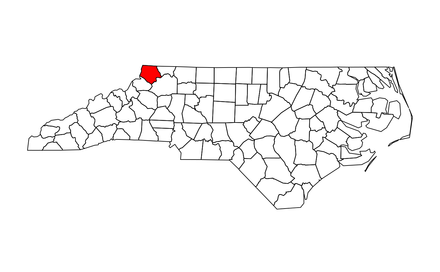
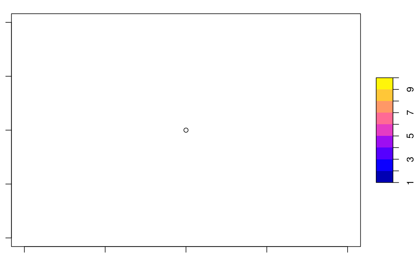
nc = st_read(system.file("gpkg/nc.gpkg", package="sf"), quiet = TRUE)
# plot single attribute, auto-legend:
plot(nc["SID74"])
# plot multiple:
plot(nc[c("SID74", "SID79")]) # better use ggplot2::geom_sf to facet and get a single legend!
# adding to a plot of an sf object only works when using reset=FALSE in the first plot:
plot(nc["SID74"], reset = FALSE)
plot(st_centroid(st_geometry(nc)), add = TRUE)
#> Warning: st_centroid does not give correct centroids for longitude/latitude data
# log10 z-scale:
plot(nc["SID74"], logz = TRUE, breaks = c(0,.5,1,1.5,2), at = c(0,.5,1,1.5,2))
# and we need to reset the plotting device after that, e.g. by
layout(1)
# when plotting only geometries, the reset=FALSE is not needed:
plot(st_geometry(nc))
plot(st_geometry(nc)[1], col = 'red', add = TRUE)
# add a custom legend to an arbitray plot:
layout(matrix(1:2, ncol = 2), widths = c(1, lcm(2)))
plot(1)
.image_scale(1:10, col = sf.colors(9), key.length = lcm(8), key.pos = 4, at = 1:10)
sf.colors(10)
#>  [1] "#0000B3FF" "#0400FFFF" "#4500FFFF" "#8500FFFF" "#C527D8FF" "#FF50AFFF"
#>  [7] "#FF7A85FF" "#FFA35CFF" "#FFCC33FF" "#FFF50AFF"