Faces recognition example using eigenfaces and SVMs

The dataset used in this example is a preprocessed excerpt of the “Labeled Faces in the Wild”, aka LFW: http://vis-www.cs.umass.edu/lfw/lfw-funneled.tgz (233MB)

# Authors: The scikit-learn developers
# SPDX-License-Identifier: BSD-3-Clause

from time import time

import matplotlib.pyplot as plt
from scipy.stats import loguniform

from sklearn.datasets import fetch_lfw_people
from sklearn.decomposition import PCA
from sklearn.metrics import ConfusionMatrixDisplay, classification_report
from sklearn.model_selection import RandomizedSearchCV, train_test_split
from sklearn.preprocessing import StandardScaler
from sklearn.svm import SVC

Download the data, if not already on disk and load it as numpy arrays

lfw_people = fetch_lfw_people(min_faces_per_person=70, resize=0.4)

# introspect the images arrays to find the shapes (for plotting)
n_samples, h, w = lfw_people.images.shape

# for machine learning we use the 2 data directly (as relative pixel
# positions info is ignored by this model)
X = lfw_people.data
n_features = X.shape[1]

# the label to predict is the id of the person
y = lfw_people.target
target_names = lfw_people.target_names
n_classes = target_names.shape[0]

print("Total dataset size:")
print("n_samples: %d" % n_samples)
print("n_features: %d" % n_features)
print("n_classes: %d" % n_classes)

Total dataset size:
n_samples: 1288
n_features: 1850
n_classes: 7

Split into a training set and a test and keep 25% of the data for testing.

X_train, X_test, y_train, y_test = train_test_split(
    X, y, test_size=0.25, random_state=42
)

scaler = StandardScaler()
X_train = scaler.fit_transform(X_train)
X_test = scaler.transform(X_test)

Compute a PCA (eigenfaces) on the face dataset (treated as unlabeled dataset): unsupervised feature extraction / dimensionality reduction

n_components = 150

print(
    "Extracting the top %d eigenfaces from %d faces" % (n_components, X_train.shape[0])
)
t0 = time()
pca = PCA(n_components=n_components, svd_solver="randomized", whiten=True).fit(X_train)
print("done in %0.3fs" % (time() - t0))

eigenfaces = pca.components_.reshape((n_components, h, w))

print("Projecting the input data on the eigenfaces orthonormal basis")
t0 = time()
X_train_pca = pca.transform(X_train)
X_test_pca = pca.transform(X_test)
print("done in %0.3fs" % (time() - t0))

Extracting the top 150 eigenfaces from 966 faces
done in 0.077s
Projecting the input data on the eigenfaces orthonormal basis
done in 0.006s

Train a SVM classification model

print("Fitting the classifier to the training set")
t0 = time()
param_grid = {
    "C": loguniform(1e3, 1e5),
    "gamma": loguniform(1e-4, 1e-1),
}
clf = RandomizedSearchCV(
    SVC(kernel="rbf", class_weight="balanced"), param_grid, n_iter=10
)
clf = clf.fit(X_train_pca, y_train)
print("done in %0.3fs" % (time() - t0))
print("Best estimator found by grid search:")
print(clf.best_estimator_)

Fitting the classifier to the training set
done in 5.375s
Best estimator found by grid search:
SVC(C=np.float64(76823.03433306457), class_weight='balanced',
    gamma=np.float64(0.0034189458230957995))

Quantitative evaluation of the model quality on the test set

print("Predicting people's names on the test set")
t0 = time()
y_pred = clf.predict(X_test_pca)
print("done in %0.3fs" % (time() - t0))

print(classification_report(y_test, y_pred, target_names=target_names))
ConfusionMatrixDisplay.from_estimator(
    clf, X_test_pca, y_test, display_labels=target_names, xticks_rotation="vertical"
)
plt.tight_layout()
plt.show()

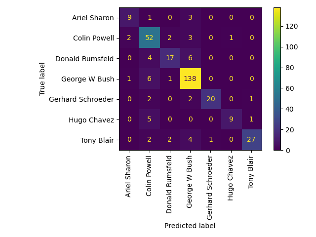
Predicting people's names on the test set
done in 0.046s
                   precision    recall  f1-score   support

     Ariel Sharon       0.75      0.69      0.72        13
     Colin Powell       0.72      0.87      0.79        60
  Donald Rumsfeld       0.77      0.63      0.69        27
    George W Bush       0.88      0.95      0.91       146
Gerhard Schroeder       0.95      0.80      0.87        25
      Hugo Chavez       0.90      0.60      0.72        15
       Tony Blair       0.93      0.75      0.83        36

         accuracy                           0.84       322
        macro avg       0.84      0.75      0.79       322
     weighted avg       0.85      0.84      0.84       322

Qualitative evaluation of the predictions using matplotlib

def plot_gallery(images, titles, h, w, n_row=3, n_col=4):
    """Helper function to plot a gallery of portraits"""
    plt.figure(figsize=(1.8 * n_col, 2.4 * n_row))
    plt.subplots_adjust(bottom=0, left=0.01, right=0.99, top=0.90, hspace=0.35)
    for i in range(n_row * n_col):
        plt.subplot(n_row, n_col, i + 1)
        plt.imshow(images[i].reshape((h, w)), cmap=plt.cm.gray)
        plt.title(titles[i], size=12)
        plt.xticks(())
        plt.yticks(())

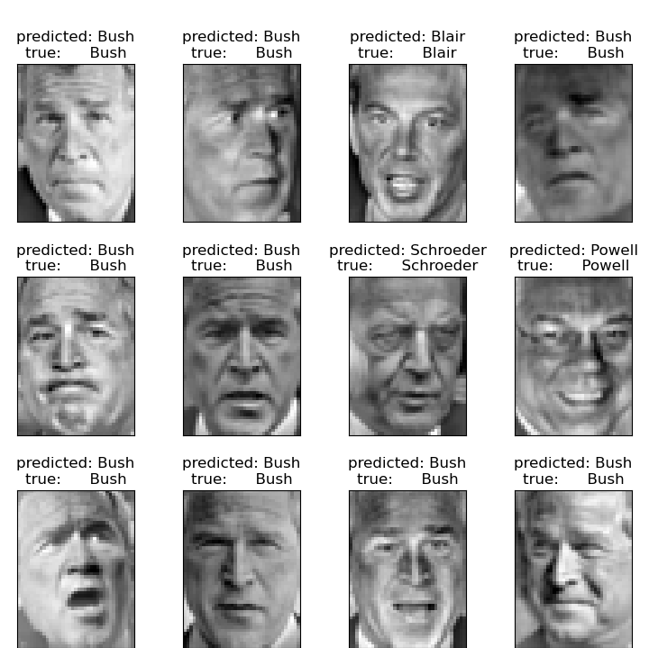
plot the result of the prediction on a portion of the test set

def title(y_pred, y_test, target_names, i):
    pred_name = target_names[y_pred[i]].rsplit(" ", 1)[-1]
    true_name = target_names[y_test[i]].rsplit(" ", 1)[-1]
    return "predicted: %s\ntrue:      %s" % (pred_name, true_name)


prediction_titles = [
    title(y_pred, y_test, target_names, i) for i in range(y_pred.shape[0])
]

plot_gallery(X_test, prediction_titles, h, w)

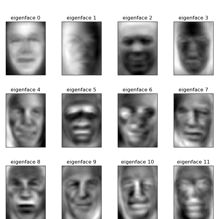
plot the gallery of the most significative eigenfaces

eigenface_titles = ["eigenface %d" % i for i in range(eigenfaces.shape[0])]
plot_gallery(eigenfaces, eigenface_titles, h, w)

plt.show()

Face recognition problem would be much more effectively solved by training convolutional neural networks but this family of models is outside of the scope of the scikit-learn library. Interested readers should instead try to use pytorch or tensorflow to implement such models.

Related examples

Topic extraction with Non-negative Matrix Factorization and Latent Dirichlet Allocation

Topic extraction with Non-negative Matrix Factorization and Latent Dirichlet Allocation

Classification of text documents using sparse features

Classification of text documents using sparse features

Online learning of a dictionary of parts of faces

Online learning of a dictionary of parts of faces

Feature agglomeration

Feature agglomeration