Section 4 Sentiment Analysis

dataDir <- "Proj2Data"

curTknsByMonth <- read.csv(paste0(dataDir, "/CoinTknsMonthly.csv"))
CommTkns <- read.csv(paste0(dataDir, "/CommTkns.csv"))

4.1 Data Shaping

To group comments and their sentiments by Coin we have to first assign this identifier to the tokens via their associated comm_id.

currTkns <- CommTkns %>%
  inner_join(curTknsByMonth[,c("Coin","Month","comm_id")], by = "comm_id")

4.1.1 get_sentiments()

nrc<- get_sentiments("nrc")

word	sentiment
abacus	trust
abandon	fear
abandon	negative
abandon	sadness
abandoned	anger
abandoned	fear

4.1.2 Sentiment Counts By Coin

#ggplot(sntmntByMonth, aes(x = Month, y = n, color = sentiment)) +
  #geom_line() +
  #facet_wrap(~Coin, scale = "free_y")

sBmPlot <- ggplot(sntmntByMonth, aes(x = as.Date(Month), y = n, group = sentiment, color = sentiment)) +
  geom_line() +
  scale_x_date(labels = date_format("%Y")) +
  facet_wrap(~Coin) +
  xlab("Month") + ylab("Number of Tokens (n)") 

ggplotly(sBmPlot)

# Quandl limits free users to 50 calls a day, so these code chunks can be run for more recent data

#pBTC <- Quandl('BITFINEX/BTCUSD')
#pETH <- Quandl('BITFINEX/ETHUSD')
#pLTC <- Quandl('BITFINEX/LTCUSD')
#pXRP <- Quandl('BITFINEX/XRPUSD')

#pBTC["Coin"] <- "BTC"
#pETH["Coin"] <- "ETH"
#pLTC["Coin"] <- "LTC"
#pXRP["Coin"] <- "XRP"

#PricesByCoin <- rbind(pBTC, pETH, pLTC, pXRP)

#To get around this call limit, we use a csv to hold the data
PricesByCoin<- read.csv(paste0(dataDir, "/pricesByCoin.csv"))

#write.csv(PricesByCoin,paste0(dataDir,"/pricesByCoin.csv"))

4.2 Price & Sentiment over Time

# function for getting Coin Price/ Sentiment vs Time graph by coin 

get_graph <- function(coin, coeff) {   # coin = "COIN_NAME", coeff = Value used to transform sentiment to match price scale on graph
  
  # get related coin data
  coinprice_data <- PricesByCoin %>% filter(Coin == coin)
  coin_sntmntByMonth <- sntmntByMonth %>% filter(Coin == coin)
  
  # reshape coin price by day data to merge high, low, last, med into one variable
  price_by_mkt_metric <- melt(coinprice_data, id = c("Date", "Coin"))
  colnames(price_by_mkt_metric)[3] <- "Mkt_Metrics"
  
  # normalize x-values for both datasets (date)
  price_by_mkt_metric$Date <- as_date(price_by_mkt_metric$Date)
  coin_sntmntByMonth$Month <- as_date(coin_sntmntByMonth$Month)
  

  # make the gg plot
  Coin_Daily_Price.plot <- price_by_mkt_metric %>%
    filter((Mkt_Metrics %in% c("High", "Low", "Last"))) %>%
    
    # ggplot setup
    ggplot(aes(x = Date)) +
    theme_minimal() +
    ggtitle(paste(coin, " Sentiment/ Price vs Time")) +
    xlab("Date") +
    theme(legend.title = element_blank())  +
    
    
    # plot price vs time lines
    geom_line(
      stat = 'identity',
      aes(
        y = value,
        linetype = Mkt_Metrics,
        color = Mkt_Metrics,
        size = Mkt_Metrics,
        alpha = Mkt_Metrics)) +
    scale_linetype_manual("Market Metrics", values = c("solid", "solid", "solid")) +
    scale_color_manual("Market Metrics", values = c('#EF9A9A', '#C5E1A5', '#212121')) +
    scale_size_manual("Market Metrics", values = c(1, 1, 0.3)) +
    scale_alpha_manual("Market Metrics", values = c(0.8, 0.8, 1)) +
    
    
    # plot sentiment bars (stacked)
    geom_bar(
      data = coin_sntmntByMonth,
      stat = 'identity',
      aes(
        x = Month,
        y = n / coeff,
        fill = sentiment)) +
    
    
    # setup y-axises
    scale_y_continuous(name = "Price (USD)",
                       sec.axis = sec_axis( ~ . * coeff,  name = "Sentiment (n)"))
  
  # convert to plotly
  Coin_Daily_Price.plotly = ggplotly(Coin_Daily_Price.plot, tooltip = c("label","x","y"))
  
  # cleans up ledgend labels
  for (i in 1:length(Coin_Daily_Price.plotly$x$data)) {
    if (!is.null(Coin_Daily_Price.plotly$x$data[[i]]$name)) {
      Coin_Daily_Price.plotly$x$data[[i]]$name =  gsub("\\(", "",
          str_split(Coin_Daily_Price.plotly$x$data[[i]]$name, ",")[[1]][1])
    }
  }
  
  Coin_Daily_Price.plot
  Coin_Daily_Price.plotly # FOR THE LIFE OF ME CANNOT FIGURE OUT HOW TO GET THE 2ND AXIS TO SHOW
}

4.2.1 BTC

get_graph("BTC", 4)

4.2.2 ETH

get_graph("ETH",20)

4.2.3 LTC

get_graph("LTC", 19)

4.2.4 XRP

get_graph("XRP", 8000)

4.3 User Sentiment

posts_by_coin <- currSntmntTkns %>% 
    group_by(Coin) %>%
    count(Coin)

users_by_coin <- currSntmntTkns %>% 
    group_by(user) %>%
    count(user)

emo_stats <- function(emote, color1, color2){
  
  users.emo <- currSntmntTkns %>% 
    filter(sentiment == emote) %>%
    count(user) 
  users.emo <- inner_join(users.emo, users_by_coin, by = "user", suffix = c(".emote", ".total")) %>%
    filter(n.total >= 500) %>%
    mutate(n.emote_porp = n.emote/n.total) %>% 
    arrange(desc(n.emote_porp) )
  
  coin.emo <- currSntmntTkns %>% 
      filter(sentiment == emote) %>%
      group_by(Coin) %>% 
      count(Coin) 
  coin.emo <- inner_join(coin.emo, posts_by_coin, by = "Coin", suffix = c(".emote", ".total")) %>%
    mutate(n.emote_porp=n.emote/n.total)
  
  #users_coin.emo TOTAL plot
  plt1 <- ggplotly(
    ggplot(coin.emo, aes(x = Coin)) +
      theme_minimal() +
      theme(panel.grid.major.x = element_blank()) +
      geom_bar(aes(y = n.emote), stat='identity', fill = color1, width = 0.5) +
      ggtitle("Total emote by coin") +
      xlab("Coin") + ylab("Emote tokens (posts.emote)") 
  )
  
  # users_coin.emo PROP plot
  plt2 <- ggplotly(
    ggplot(coin.emo, aes(x = Coin)) +
      theme_minimal() +
      theme(panel.grid.major.x = element_blank()) +
      geom_bar(aes(y = n.emote_porp), stat='identity', fill = color2, width = 0.5) +
      ggtitle("Proportion of emote by coin") +
      xlab("Coin") + ylab("Emote tokens (posts.emote/ posts.total)") 
  )
  
  return(list(as_tibble(users.emo), plt1, plt2))
}

4.3.1 Angriest

Angriest users

ang <- emo_stats("anger", "#F1948A", "#E6B0AA")
head(ang[[1]])

## # A tibble: 6 x 4
##   user              n.emote n.total n.emote_porp
##   <chr>               <int>   <int>        <dbl>
## 1 adamlh                 98     540        0.181
## 2 tippr                 392    2580        0.152
## 3 HughHonee              99     675        0.147
## 4 Cryptopricedrops      158    1120        0.141
## 5 DontMicrowaveCats      90     650        0.138
## 6 ggekko999             221    1599        0.138

ang[[2]]

ang[[3]]

4.3.2 Happiest

Top most joyful/ positive users

hap <- emo_stats(c("joy", "positive"), "#F7DC6F", "#FCF3CF")
head(hap[[1]])

## # A tibble: 6 x 4
##   user              n.emote n.total n.emote_porp
##   <chr>               <int>   <int>        <dbl>
## 1 NotGonnaGetBanned     962    2886        0.333
## 2 Vincents_keyboard     300    1107        0.271
## 3 Tribal_Tech           397    1466        0.271
## 4 JohndeBoer           1187    4472        0.265
## 5 cryptolicious501      163     674        0.242
## 6 Hanzburger            205     851        0.241

hap[[2]]

hap[[3]]

4.3.3 Saddest

Top saddest/ most negative users

sad <- emo_stats(c("negative", "sad"), "#5499C7", "#D4E6F1")
head(sad[[1]])

## # A tibble: 6 x 4
##   user              n.emote n.total n.emote_porp
##   <chr>               <int>   <int>        <dbl>
## 1 japsock                96     556        0.173
## 2 brobits               117     875        0.134
## 3 ebringer              112     880        0.127
## 4 DontMicrowaveCats      80     650        0.123
## 5 Cryptopricedrops      136    1120        0.121
## 6 Hypocriciety          110     919        0.120

sad[[2]]

sad[[3]]

4.4 Descriptive Statistics

ggplot(sntmntByMonth, aes(x = Coin, fill = Coin)) + geom_bar() +  ggtitle("Distribution of Coin Types")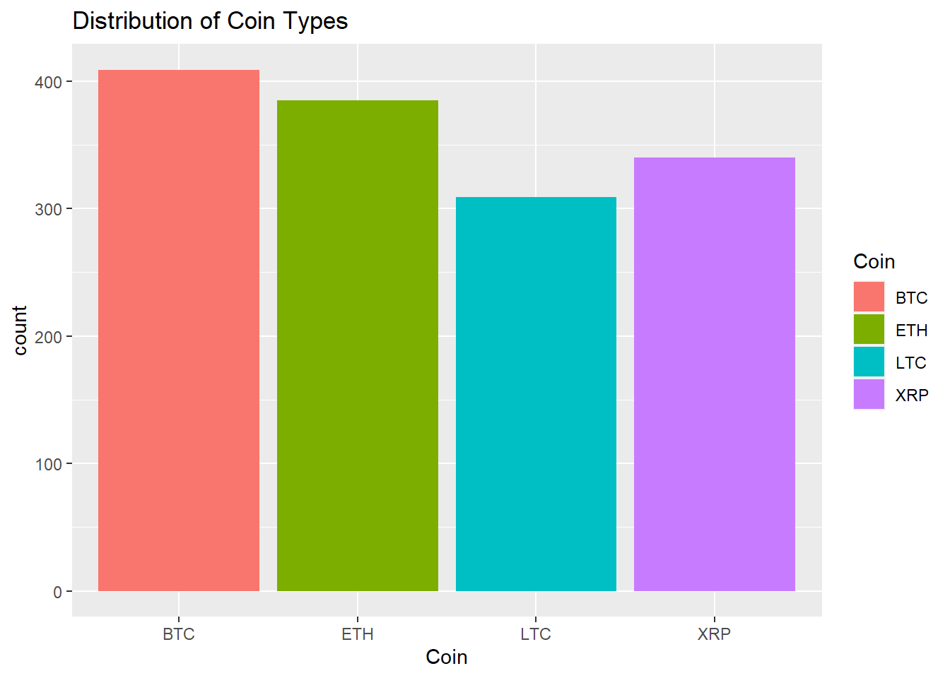

ggplot(sntmntByMonth, aes(x = sentiment, fill = sentiment)) + geom_bar() +  ggtitle("Distribution Sentiments Among All Coins")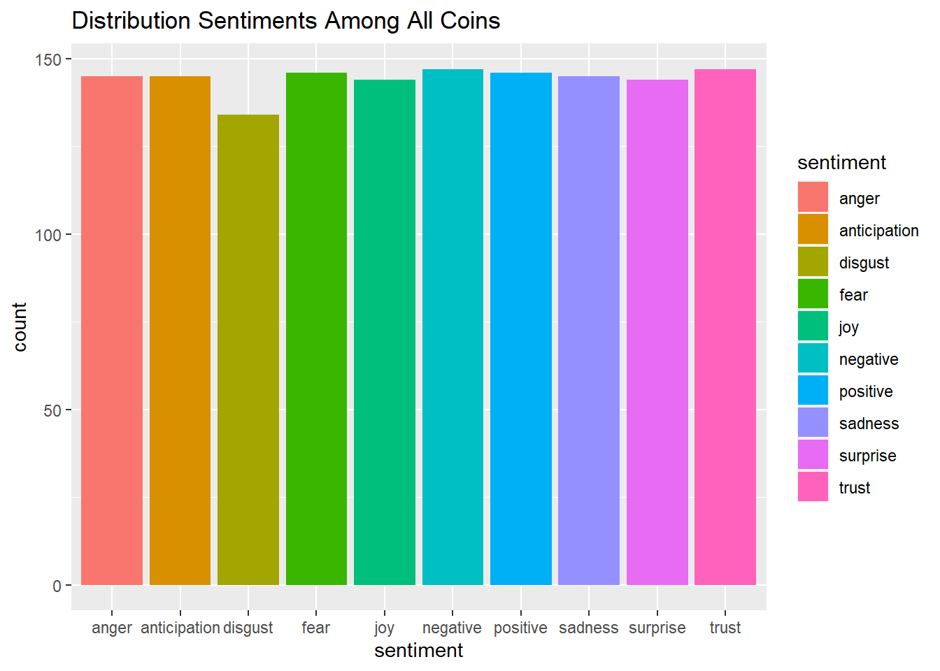

ggplot(sntmntByMonth, aes(x = Month, fill = Month)) + geom_bar() +  ggtitle("Number of Sentiment Types for Each Month")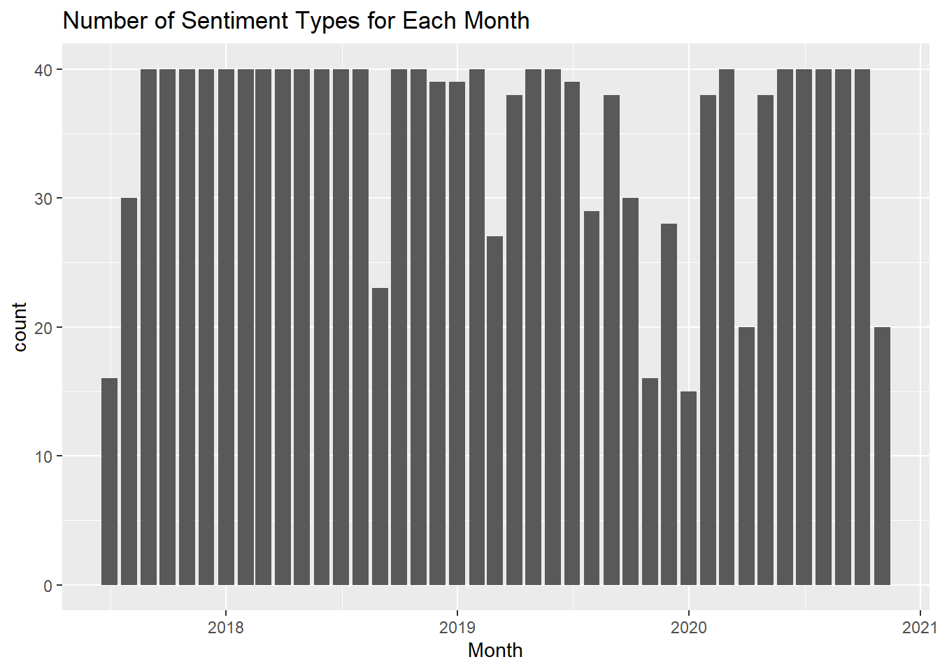

ggplot(sntmntByMonth, aes(x = sentiment, y = n, color = Coin)) + geom_point() +  ggtitle("Popularity of Each Sentiment Among Coin Type")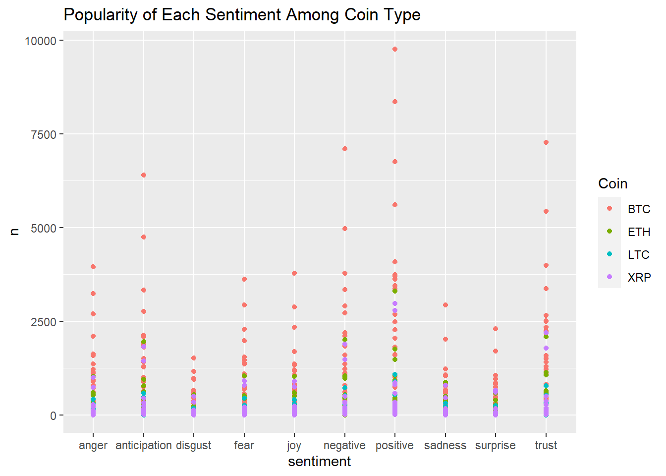

4.5 Most Abundant Sentiment Over Time

aggSent <- function(pop.df, n, m, coindf, unevenStep = FALSE){
  k = 1
  j = 1
  for (i in 1:n){
    if(coindf[i,2] == m[j]){
      if(coindf[i,4] > pop.df[j,3]){
        pop.df[j,3] = coindf[i,4]
        pop.df[j,2] = coindf[i,3]
        pop.df[j,4] = pop.df[j,4] + coindf[i,4]
        pop.df[j,5] = pop.df[j,3] / pop.df[j,4]
      }
    }

    k = k + 1
    
    
    
    
    if(k == 11){
      j = j + 1
      k = 1
    }
  }
  return(pop.df)
}

df <- sntmntByMonth

df <- na.omit(df)

# create a new dataframe for each coin

btc <- df[which(df$Coin == "BTC"),]


btc_m <- unique(btc$Month)

btc_n <- nrow(btc)

n <- length(btc_m)
sentiment <- rep("x", n)


btc.pop.df <- data.frame(btc_m, sentiment,0, 0, 0)

btc.pop.df <- aggSent(btc.pop.df, btc_n, btc_m, btc)

# ETH

eth <- df[which(df$Coin == "ETH"),]
eth_m <-  unique(eth$Month)

eth_n <- nrow(eth)

n <- length(eth_m)
sentiment <- rep("x", n)

eth.pop.df <- data.frame(eth_m, sentiment,0, 0, 0)


#eth.pop.df <- aggSent(eth.pop.df, eth_n, eth_m, eth, unevenStep = TRUE)


#eth.pop.df

j <- 1

for(i in 1:eth_n){
  if(i > 1){
    prevM <- eth[i-1, 2]
    month <- eth[i,2]
  
    if(month != prevM){
      j <- j + 1
    }
    
  }
  
  if(eth[i,2] == eth_m[j]){
      if(eth[i,4] > eth.pop.df[j,3]){
        eth.pop.df[j,3] = eth[i,4]
        eth.pop.df[j,2] = eth[i,3]
        eth.pop.df[j,4] = eth.pop.df[j,4] + eth[i,4]
        eth.pop.df[j,5] = eth.pop.df[j,3] / eth.pop.df[j,4]
      }
    
  }
  
}



#xrp <- df[which(df$Coin == "XRP"),]

#eth.pop.df



ltc <- df[which(df$Coin == "LTC"),]

ltc_m <-  unique(ltc$Month)

ltc_n <- nrow(ltc)

n <- length(ltc_m)
sentiment <- rep("x", n)

ltc.pop.df <- data.frame(ltc_m, sentiment,0, 0, 0)

j <- 1

for(i in 1:ltc_n){
  if(i > 1){
    prevM <- ltc[i-1, 2]
    month <- ltc[i,2]
  
    if(month != prevM){
      j <- j + 1
    }
    
  }
  
  if(ltc[i,2] == ltc_m[j]){
      if(ltc[i,4] > ltc.pop.df[j,3]){
        ltc.pop.df[j,3] = ltc[i,4]
        ltc.pop.df[j,2] = ltc[i,3]
        ltc.pop.df[j,4] = ltc.pop.df[j,4] + ltc[i,4]
        ltc.pop.df[j,5] = ltc.pop.df[j,3] / ltc.pop.df[j,4]
      }
    
  }
  
  
}
ltc.pop.df

##         ltc_m    sentiment   X0 X0.1      X0.2
## 1  2017-08-01     positive   26   52 0.5000000
## 2  2017-09-01     positive   67  116 0.5775862
## 3  2017-10-01     positive   54   97 0.5567010
## 4  2017-11-01     positive  229  442 0.5180995
## 5  2017-12-01     positive 1077 2800 0.3846429
## 6  2018-01-01     positive  886 2164 0.4094270
## 7  2018-02-01     positive  531 1239 0.4285714
## 8  2018-03-01     positive  161  466 0.3454936
## 9  2018-04-01     positive  263  715 0.3678322
## 10 2018-05-01     positive  134  260 0.5153846
## 11 2018-06-01     positive   56   98 0.5714286
## 12 2018-07-01     positive   31   56 0.5535714
## 13 2018-08-01     positive   38   98 0.3877551
## 14 2018-10-01     positive   21   34 0.6176471
## 15 2018-11-01     positive    8   20 0.4000000
## 16 2018-12-01     negative   11   18 0.6111111
## 17 2019-01-01     positive   14   31 0.4516129
## 18 2019-02-01     positive   18   46 0.3913043
## 19 2019-04-01     positive    7   12 0.5833333
## 20 2019-05-01     positive   18   55 0.3272727
## 21 2019-06-01     positive  216  381 0.5669291
## 22 2019-07-01     positive   14   35 0.4000000
## 23 2019-09-01     positive    8   15 0.5333333
## 24 2019-11-01         fear    2    3 0.6666667
## 25 2020-02-01     negative    4    6 0.6666667
## 26 2020-03-01     positive   78  204 0.3823529
## 27 2020-05-01 anticipation    5    6 0.8333333
## 28 2020-06-01     positive  127  229 0.5545852
## 29 2020-07-01     positive   14   23 0.6086957
## 30 2020-08-01     positive   22   45 0.4888889
## 31 2020-09-01     positive   34   82 0.4146341
## 32 2020-10-01     positive   43   77 0.5584416

xrp <- df[which(df$Coin == "XRP"),]

xrp_m <-  unique(xrp$Month)

xrp_n <- nrow(xrp)

n <- length(xrp_m)
sentiment <- rep("x", n)

xrp.pop.df <- data.frame(xrp_m, sentiment,0, 0, 0)

j <- 1


for(i in 1:xrp_n){
  if(i > 1){
    prevM <- xrp[i-1, 2]
    month <- xrp[i,2]
  
    if(month != prevM){
      j <- j + 1
    }
  }
  if(xrp[i,2] == xrp_m[j]){
      if(xrp[i,4] > xrp.pop.df[j,3]){
        xrp.pop.df[j,3] = xrp[i,4]
        xrp.pop.df[j,2] = xrp[i,3]
        xrp.pop.df[j,4] = xrp.pop.df[j,4] + xrp[i,4]
        xrp.pop.df[j,5] = xrp.pop.df[j,3] / xrp.pop.df[j,4]
      }
  }
}
xrp.pop.df

##         xrp_m sentiment   X0 X0.1      X0.2
## 1  2017-09-01  positive   42  110 0.3818182
## 2  2017-10-01  positive   27   43 0.6279070
## 3  2017-11-01  positive   53  113 0.4690265
## 4  2017-12-01  positive 2784 6425 0.4333074
## 5  2018-01-01  positive 2969 7678 0.3866892
## 6  2018-02-01  positive  802 1483 0.5407957
## 7  2018-03-01  positive  858 1943 0.4415852
## 8  2018-04-01  positive  165  363 0.4545455
## 9  2018-05-01  positive  571 1346 0.4242199
## 10 2018-06-01  positive  339  822 0.4124088
## 11 2018-07-01  positive   35   64 0.5468750
## 12 2018-08-01  positive   16   33 0.4848485
## 13 2018-09-01     anger    2    2 1.0000000
## 14 2018-10-01  positive   18   41 0.4390244
## 15 2018-11-01  positive  114  266 0.4285714
## 16 2018-12-01  positive  199  430 0.4627907
## 17 2019-01-01  negative   11   18 0.6111111
## 18 2019-02-01  positive   39  141 0.2765957
## 19 2019-03-01  negative   27   43 0.6279070
## 20 2019-04-01  positive   17   30 0.5666667
## 21 2019-05-01  positive   71  144 0.4930556
## 22 2019-06-01  positive  285  707 0.4031117
## 23 2019-07-01  positive   12   21 0.5714286
## 24 2019-08-01  positive   10   22 0.4545455
## 25 2019-09-01  positive   28   67 0.4179104
## 26 2019-10-01  positive   33   74 0.4459459
## 27 2019-12-01  positive  191  428 0.4462617
## 28 2020-02-01  negative   12   25 0.4800000
## 29 2020-03-01  positive   63  179 0.3519553
## 30 2020-05-01  positive  232  389 0.5964010
## 31 2020-06-01  positive   33   86 0.3837209
## 32 2020-07-01  positive   24   77 0.3116883
## 33 2020-08-01  negative   22   43 0.5116279
## 34 2020-09-01  positive   10   17 0.5882353
## 35 2020-10-01  negative   26   45 0.5777778

4.6 Plots of Top Sentiment Over Time

ggplot(data = btc.pop.df, aes(x=btc_m, y = X0.2, group = 1, color = sentiment))+
  geom_line()+
  geom_point() + 
  theme(axis.text.x = element_text(angle = 60, hjust = 1)) + ggtitle("Most Common Sentiment Over Time For BTC") + xlab("Month") + ylab("Proportion of Sentiment")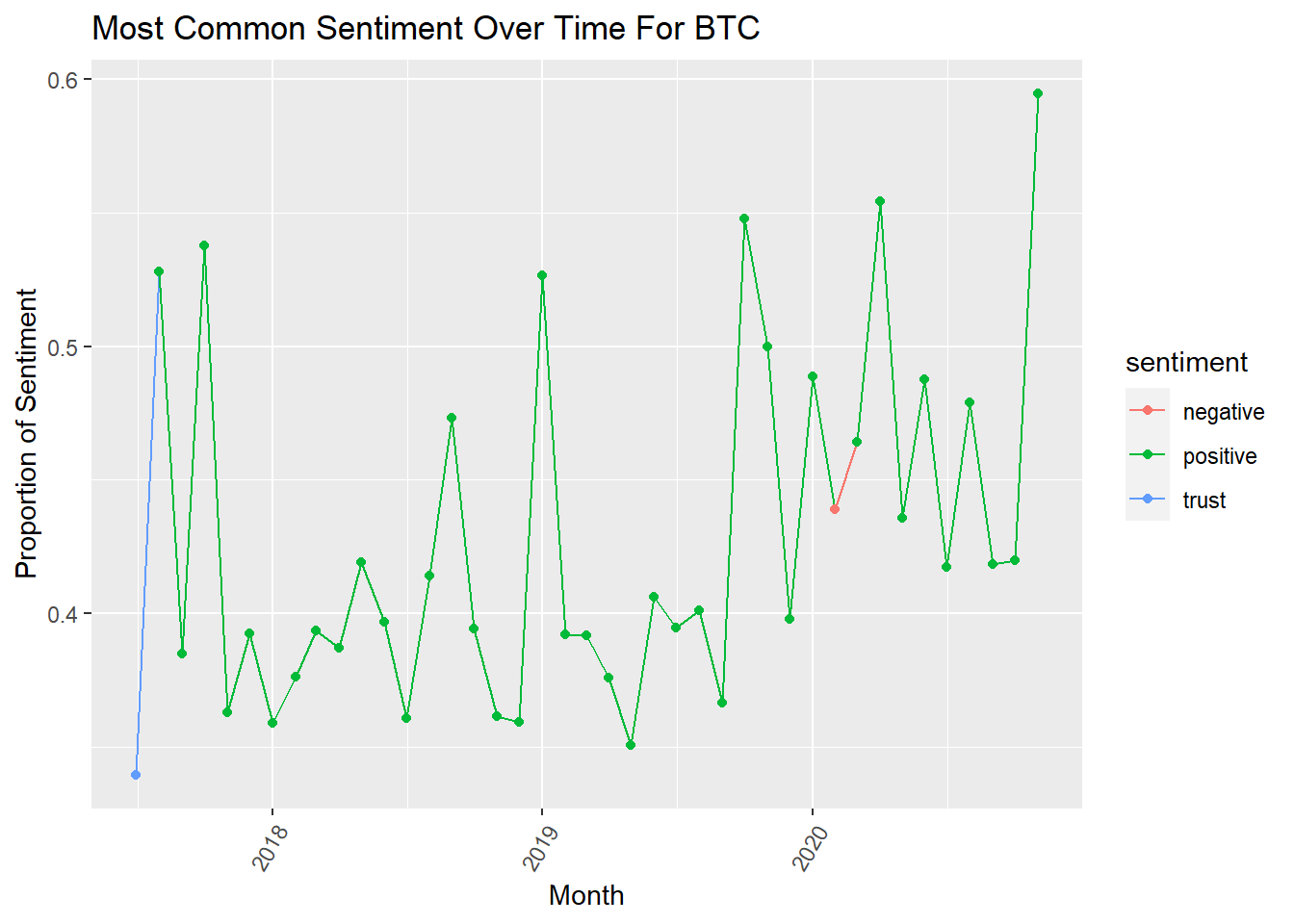

ggplot(data = eth.pop.df, aes(x=eth_m, y = X0.2, group = 1, color = sentiment))+
  geom_line()+
  geom_point() + 
  theme(axis.text.x = element_text(angle = 60, hjust = 1)) + ggtitle("Most Common Sentiment Over Time For ETH") + xlab("Month") + ylab("Proportion of Sentiment")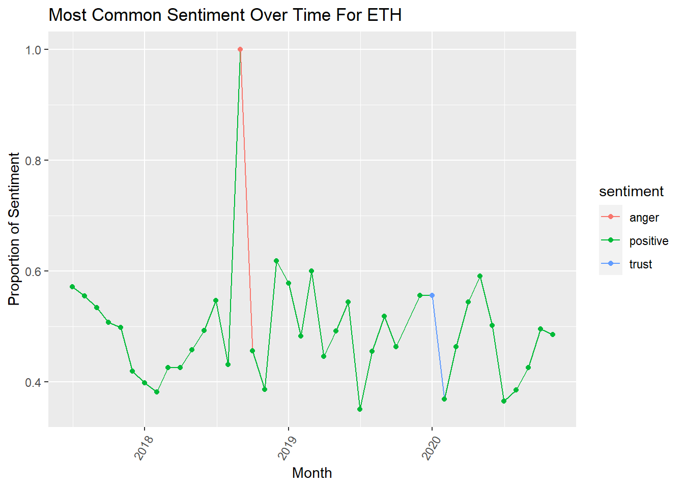

ggplot(data = ltc.pop.df, aes(x=ltc_m, y = X0.2, group = 1, color = sentiment))+
  geom_line()+
  geom_point() + 
  theme(axis.text.x = element_text(angle = 60, hjust = 1)) + ggtitle("Most Common Sentiment Over Time For LTC") + xlab("Month") + ylab("Proportion of Sentiment")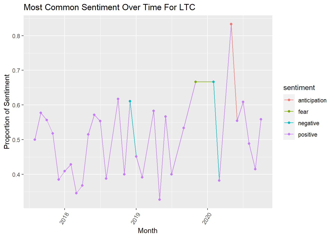

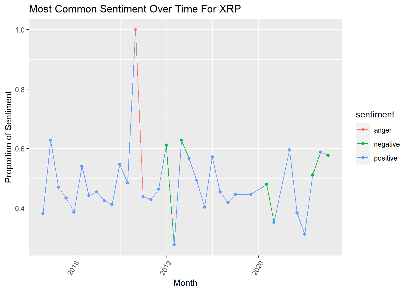
ggplot(data = xrp.pop.df, aes(x=xrp_m, y = X0.2, group = 1, color = sentiment))+
  geom_line()+
  geom_point() + 
  theme(axis.text.x = element_text(angle = 60, hjust = 1)) + ggtitle("Most Common Sentiment Over Time For XRP") + xlab("Month") + ylab("Proportion of Sentiment")