Categorisation
Categorisation is another useful application for web data you can perform in R.
In this case, we are looking to how we can classify web data to create different segments created by the data (as opposed to what you may pick), or if you give categories to R if they can help you define those categories via other metrics.
Decision trees
Decision trees are typically read top to bottom, and represent where the model thinks you can split your data. As you move down
library(knitr) # used for kable that makes nice RMarkdown tables
web_data <- read.csv("./data/gadata_example_2.csv", stringsAsFactors = FALSE)
kable(head(web_data[-1]), row.names = FALSE)| date | channelGrouping | deviceCategory | sessions | pageviews | entrances | bounces |
|---|---|---|---|---|---|---|
| 2016-01-01 | (Other) | desktop | 19 | 23 | 19 | 15 |
| 2016-01-01 | (Other) | mobile | 112 | 162 | 112 | 82 |
| 2016-01-01 | (Other) | tablet | 24 | 41 | 24 | 19 |
| 2016-01-01 | Direct | desktop | 133 | 423 | 133 | 61 |
| 2016-01-01 | Direct | mobile | 345 | 878 | 344 | 172 |
| 2016-01-01 | Direct | tablet | 126 | 237 | 126 | 77 |
library(dplyr) # data transformation
cats <- web_data %>% select(deviceCategory, channelGrouping, sessions)

kable(head(cats), row.names = FALSE)| deviceCategory | channelGrouping | sessions |
|---|---|---|
| desktop | (Other) | 19 |
| mobile | (Other) | 112 |
| tablet | (Other) | 24 |
| desktop | Direct | 133 |
| mobile | Direct | 345 |
| tablet | Direct | 126 |
library(rpart) # creates decision trees

tree <- rpart(deviceCategory ~ ., cats)
plot(tree)
text(tree)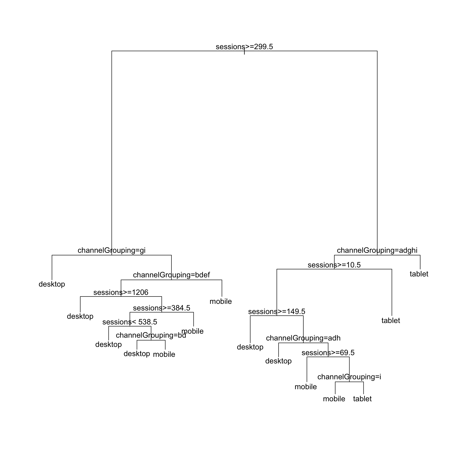
The labels are a bit obscure as they abbreviate the channel names.
The package rpart.plot makes the plots much nicer and easier to interpret:
library(rpart.plot)  # pretty trees
rpart.plot(tree, type=1)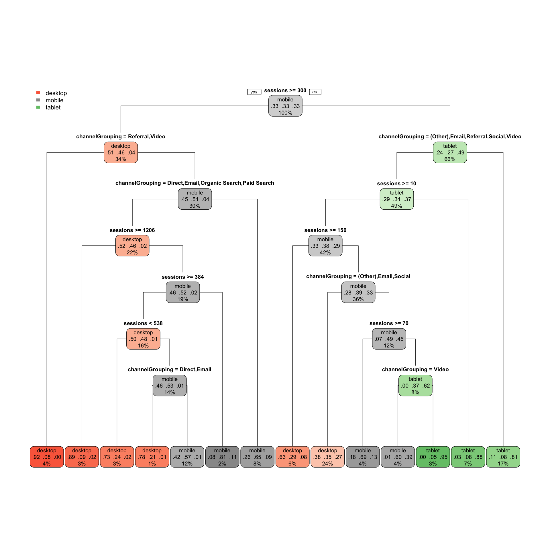
Each node shows:
- the predicted class (Much worse, worse, …, Much better),
- the predicted probability of each class,
- the percentage of observations in the node (note not % of sessions)
From this you can see from this data at a glance that for sessions under 300, Tablet traffic was not search related at all, favouring Email, Referral, Social and Video.
Machine learning
Categorisation is a use case for machine learning, as it utilises self-validation checks to check your categorisatons. Two methods are talked about in more length in the blog post, “Introduction to Machine Learning with Web Analytics: Random Forests and K-Means”.