Google Analytics Data Explorer
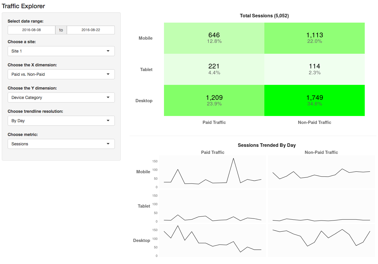
Example 2: Google Analytics 2-D data explorer
This was Tim’s first web-based, interactive R applications. In hindsight…it was ambitious. It’s available at https://gilligan.shinyapps.io/ga_explorer_demo/.
Some keys to the underlying functionality used to build this:
- The
RGApackage – one of several packages available for pulling data from Google Analytics - The
shinypackage – Shiny is a package that makes R scripts interactive and web-based. - The
ggplot2package – the visualizations are all built using the plotting capabilities of ggplot2
The Code
This code does not use best practices for coding in general or for R in particular. But…it works. And, in this case, that’s what mattered. The typical way to build Shiny apps is to have two scripts: one defines the front end (ui.R) and the other defines the behind-the-scenes work (server.R). They reference each other, and it can be confusing as to how exactly that happens.
ui.R
library(shiny)

shinyUI(fluidPage(

  # This feels a little hacky, but the default <h2> is just too big.
  HTML('<style type="text/css">h2 {font-size: 150%;}</style>'),

  # Application title
  titlePanel(
    "Traffic Explorer"),

  fluidRow(
    column(4,wellPanel(

      # 'start' is hacked to default to the last full months; this needs to be cleaned up
      dateRangeInput('dateRange',
                     label = 'Select date range:',
                     start = Sys.Date()-15, end = Sys.Date()-1
      ),

      # Brand Selector
      uiOutput("brandSelector"),

      # X Dimension Selector
      uiOutput("dimXSelector"),

      # Y Dimension Selector
      uiOutput("dimYSelector"),

       # Date Granularity
      uiOutput("granularitySelector"),

      # Metric Selector
      uiOutput("metricSelector")

    )),

    column(8,plotOutput("plotTotal"),
           hr(),
           plotOutput("plotTrends"))
    )))
server.R
library(shiny) # Package for making this thing run
library(RGA) # Package for getting GA data
library(ggplot2) # Package for rendering the graphics
library(dplyr) # Efficient manipulation of the data output.
library(scales) # To allow numbers to be formatted with commas and improved date formatting

# Authorize the Google Analytics account
ga_token <- authorize(client.id = "[insert Google Analytics API client ID]",
                      client.secret = "[insert Google Analytics API client secret]",
                      cache = "token")

#########################
# Configuration and loading of options
#########################

# List of sites to choose from. This includes the name for the site as well as
# the view ID for the site. Replace the values in brackets (and the brackets) with
# site names and corresponding view IDs. This list can be as long or as short as you
# want it to be.
brandMaster <- list("[Site 1 Display Name]"="[View ID]",
                    "[Site 2 Display Name]"="[View ID]",
                    "[Site 3 Display Name]"="[View ID]")

########################
# No additional edits are REQUIRED after this point in order for the app to work. You certainly
# CAN make additional edits, but only the values in brackets above must have updated valued.
########################

# Define the segment snippets. This is just a matrix where each row has the group name in the 1st column,
# the individual segment name in the second column, and the segment definition in the third column.
# The segment definitions use GA's "dynamic segment" syntax. NOTE: the "sessions::" or "users::"
# component of the segment definition is NOT included here because that gets added later. This
# script combines the snippets to make a segment for each "box" on the grid of results. Generally
# speaking, the segment snippets within any individual group should be mutually exclusive. Otherwise,
# the results will be tricky to interpret. Feel free to add additional groups/segments to this list!
segMaster <- matrix(c("Paid vs. Non-Paid","Paid Traffic",
                      "condition::ga:channelGrouping=~(Paid.Search)|(Display)|(Video)|(Social)|(Email)|(Other)"),1,3)
segMaster <- rbind(segMaster,c("Paid vs. Non-Paid","Non-Paid Traffic",
                               "condition::ga:channelGrouping=~(Organic.Search)|(Direct)|(Referral)"))
segMaster <- rbind(segMaster,c("Device Category","Desktop",
                               "condition::ga:deviceCategory==desktop"))
segMaster <- rbind(segMaster,c("Device Category","Tablet",
                               "condition::ga:deviceCategory==tablet"))
segMaster <- rbind(segMaster,c("Device Category","Mobile",
                               "condition::ga:deviceCategory==mobile"))
segMaster <- rbind(segMaster,c("New vs. Returning","New Visitors",
                               "condition::ga:userType==New Visitor"))
segMaster <- rbind(segMaster,c("New vs. Returning","Returning Visitors",
                               "condition::ga:userType==Returning Visitor"))

colnames(segMaster) <- c("group","segName","segDef")

# Set up the data granularity options
granularityMaster <- list("By Day"="ga:date",
                          "By Week"="ga:week",
                          "By Month"="ga:yearMonth")

# Set up the available metrics. With this version of the code, the only metrics that will be reliable
# are ones that are additive. In other words, ga:users will pull in data...but it will be misleading.
metricMaster <- list("Sessions"="ga:sessions",
                     "Page Views"="ga:pageviews",
                     "Bounces"="ga:bounces")

# Initialize a list that will hold the detailed data.
##### QUESTION: Is this needed? Is this where it should be? #####
allData <- data.frame(brand=character(0),viewId=character(0),segment.X=character(0),
                      segment.Y=character(0), date=character(0),metric=numeric(0))

# Define the base theme for the plots. Each plot will selectively override this stuff as needed
baseTheme <- theme(plot.title = element_text(face = "bold", size=16, colour="gray10"),
                   axis.line = element_blank(),
                   axis.text = element_text(face = "bold", size = 15, colour = "gray40"),
                   axis.ticks = element_blank(),
                   panel.grid.major = element_blank(),
                   panel.grid.minor = element_blank(),
                   panel.border = element_blank(),
                   panel.background = element_rect(fill="gray99"),
                   legend.position = "none",
                   strip.background = element_blank(),
                   strip.text = element_text(face = "bold", size = 15, colour = "gray40"))


shinyServer(function(input, output) {

  ######################################################################################
  # Set up Input Selectors
  ######################################################################################

  # Set up the list to allow the user to choose which brand/site to use
  output$brandSelector <- renderUI ({
    brands <- names(brandMaster)  # Grab just the brands (not the view IDs)
    defaultBrand <- brands[1] # Set the brand that is selected by default as the first one in the list
    selectInput("brand", label = "Choose a site:",
                choices = brands,
                selected = defaultBrand)
  })

  # Set up the list to allow the user to choose what to use for the Y dimension
  output$dimXSelector <- renderUI ({
    dimOptions <- unique(segMaster[,1])
    defaultDimX <- dimOptions[1] # Set the group that is selected by default as the first one in the list
    selectInput("dimX", label = "Choose the X dimension:",
                choices = dimOptions,
                selected = defaultDimX)
  })

  # Set up the list to allow the user to choose what to use for the Y dimension
  output$dimYSelector <- renderUI ({
    dimOptions <- unique(segMaster[,1])
    defaultDimY <- dimOptions[2] # Set the group that is selected by default as the first one in the list
    selectInput("dimY", label = "Choose the Y dimension:",
                choices = dimOptions,
                selected = defaultDimY)
  })

  # Set up the list to allow the user to choose the data granularity for the trendlines
  output$granularitySelector <- renderUI ({
    granularityOptions <- names(granularityMaster)  # Grab just the brands (not the view IDs)
    # Set the granularity that is selected by default as the first one in the list
    defaultGranularity <- granularityOptions[1]
    selectInput("granularity", label = "Choose trendline resolution:",
                choices = granularityOptions,
                selected = defaultGranularity)
  })

  # Set up the list to allow the user to choose the metric to use for the results
  output$metricSelector <- renderUI ({
    metricOptions <- names(metricMaster)  # Grab just the brands (not the view IDs)
    defaultMetric <- metricOptions[1] # Set the metric that is selected by default as the 1st in the list
    selectInput("metric", label = "Choose metric:",
                choices = metricOptions,
                selected = defaultMetric)
  })

  #############################
  # Main function to pull the data based on selected inputs.
  #############################

  getDataFromGA <- reactive({

    req(input$brand)  ########## Do I need this if I have a default value set?

    c.brandName <- input$brand
    c.viewId <- brandMaster[[input$brand]]
    c.metric <- metricMaster[[input$metric]]
    c.granularity <- granularityMaster[[input$granularity]]
    c.dimXlabel <- input$dimX
    c.dimYlabel <- input$dimY

    segmentNames.X <- segMaster[segMaster[,"group"]==c.dimXlabel,2]
    segmentDefinitions.X <- segMaster[segMaster[,"group"]==c.dimXlabel,3]

    segmentNames.Y <- segMaster[segMaster[,"group"]==c.dimYlabel,2]
    segmentDefinitions.Y <- segMaster[segMaster[,"group"]==c.dimYlabel,3]

    # Pull data for each segment. This is just a loop that goes through and makes successive calls to
    # GA and then builds out the data frame with the data.
    for (j in 1:length(segmentDefinitions.X)) {

      # Get the segment details for the x-axis
      c.segmentName.X <- segmentNames.X[j]
      c.segmentDefinition.X <- segmentDefinitions.X[j]

      for (i in 1:length(segmentDefinitions.Y)) {

        # Get the segment details for the x-axis
        c.segmentName.Y <- segmentNames.Y[i]
        c.segmentDefinition.Y <- segmentDefinitions.Y[i]

        # Combine the two segments. This is, basically, the segment to get "1 box" on the
        # heatmap (and the trended detail)
        c.segmentDefinition.XY <- paste(c("sessions::",c.segmentDefinition.X,";",
                                          c.segmentDefinition.Y),collapse="")

        # Get the users who visit from that segment -- by month
        gaData <- get_ga(profileId = c.viewId,
                         start.date = input$dateRange[1], end.date = input$dateRange[2],
                         metrics = c.metric, dimensions = c.granularity, sort = NULL, filters = NULL,
                         segment = c.segmentDefinition.XY, samplingLevel = "HIGHER_PRECISION",
                         start.index = NULL, max.results = NULL, include.empty.rows = NULL,
                         fetch.by = NULL, ga_token)
        # Combine the data with the meta data about it
        tempData <- data.frame(brand = c.brandName, viewId=c.viewId,
                               segment.X=c.segmentName.X, segment.Y=c.segmentName.Y,
                               date = gaData[,1], metric = gaData[,2])
        # Add the data to the data frame
        allData <- rbind(allData,tempData)
      }
    }

    # Reset the column names just to make sure they're right. The absence of this was causing
    # the last column to not be named "metric" in some cases, which caused issues later in the code.
    colnames(allData) <- c("brand",   "viewId", "segment.X", "segment.Y", "date", "metric")
    return(allData)

  })

  ###############################
  # Plot the data
  ###############################

  # Make the heatmap plot
  output$plotTotal <- renderPlot({
    allData <- getDataFromGA()

    #   Collapse the values to remove the monthly breakdown
    allData_total <- allData %>% group_by(segment.X, segment.Y) %>%
      summarise(metric = sum(metric)) %>%
      ungroup()

    # We're going to display the % of total, too, so going ahead and calculating
    # the total
    metricTotal <- sum(allData_total$metric)

    # Plot the result total
    ggplot(allData_total,aes(x = segment.X, y = segment.Y, fill = metric)) +
      geom_tile() + scale_fill_gradient(low="white", high="green") +
      geom_text(aes(fill = allData_total$metric, label = comma(allData_total$metric)),
                size=8, colour = "black", position = position_nudge(y = 0.1)) +
      geom_text(aes(fill = allData_total$metric, label = percent(allData_total$metric/metricTotal)),
                size=6, colour = "gray40", position = position_nudge(y = -0.1)) +
      labs(title = paste(c("Total " ,input$metric," (",comma(sum(allData_total$metric)),")"),collapse="")) +
      baseTheme + theme(panel.background = element_blank()) +
      scale_x_discrete("") +
      scale_y_discrete("")
  })

  # Plot trendlines for each block.
  output$plotTrends <- renderPlot({
    allData <- getDataFromGA()
    # Reverse the order of the y-axis factors so the facets will appear in the
    # same order as the heatmap totals above. This seemed like it was going to be
    # unbelievably messy to do... but this does it.
    allData$segment.Y <- factor(allData$segment.Y, levels=rev(levels(allData$segment.Y)))

    ggplot(data = allData, mapping = aes(x = date, y = metric, group=1)) +
      geom_line() +
      facet_grid(segment.Y ~ segment.X, switch="y") +
      baseTheme +
      labs(title = paste(c(input$metric," Trended " ,input$granularity),collapse="")) +
      scale_y_continuous(name="", labels = comma) +
      theme(axis.title = element_blank(),axis.text.x = element_blank(),
            strip.text.y = element_text(angle=180, hjust=1),
            axis.text = element_text(face = "plain", size = 11, colour = "gray40"))
  })

})