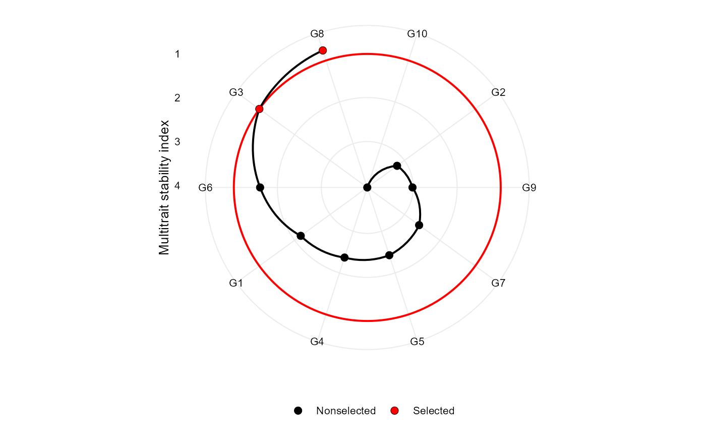
Plot the multi-trait stability index

Makes a radar plot showing the multitrait stability index proposed by Olivoto et al. (2019)

Usage

# S3 method for mtsi
plot(
  x,
  SI = 15,
  type = "index",
  position = "fill",
  genotypes = "selected",
  title = TRUE,
  radar = TRUE,
  arrange.label = FALSE,
  x.lab = NULL,
  y.lab = NULL,
  size.point = 2.5,
  size.line = 0.7,
  size.text = 10,
  width.bar = 0.75,
  n.dodge = 1,
  check.overlap = FALSE,
  invert = FALSE,
  col.sel = "red",
  col.nonsel = "black",
  legend.position = "bottom",
  ...
)

Arguments

x: An object of class mtsi
SI: An integer (0-100). The selection intensity in percentage of the total number of genotypes.
type: The type of the plot. Defaults to "index". Use type = "contribution" to show the contribution of each factor to the MGIDI index of the selected genotypes.
position: The position adjustment when type = "contribution". Defaults to "fill", which shows relative proportions at each trait by stacking the bars and then standardizing each bar to have the same height. Use position = "stack" to plot the MGIDI index for each genotype.
genotypes: When type = "contribution" defines the genotypes to be shown in the plot. By default (genotypes = "selected" only selected genotypes are shown. Use genotypes = "all" to plot the contribution for all genotypes.)
title: Logical values (Defaults to TRUE) to include automatically generated titles.
radar: Logical argument. If true (default) a radar plot is generated after using coord_polar().
arrange.label: Logical argument. If TRUE, the labels are arranged to avoid text overlapping. This becomes useful when the number of genotypes is large, say, more than 30.
x.lab, y.lab: The labels for the axes x and y, respectively. x label is set to null when a radar plot is produced.
size.point: The size of the point in graphic. Defaults to 2.5.
size.line: The size of the line in graphic. Defaults to 0.7.
size.text: The size for the text in the plot. Defaults to 10.
width.bar: The width of the bars if type = "contribution". Defaults to 0.75.
n.dodge: The number of rows that should be used to render the x labels. This is useful for displaying labels that would otherwise overlap.
check.overlap: Silently remove overlapping labels, (recursively) prioritizing the first, last, and middle labels.
invert: Logical argument. If TRUE, rotate the plot.
col.sel: The colour for selected genotypes. Defaults to "red".
col.nonsel: The colour for nonselected genotypes. Defaults to "black".
legend.position: The position of the legend.
...: Other arguments to be passed from ggplot2::theme().

Value

An object of class gg, ggplot.

References

Olivoto, T., A.D.C. L\'ucio, J.A.G. da silva, B.G. Sari, and M.I. Diel. 2019. Mean performance and stability in multi-environment trials II: Selection based on multiple traits. Agron. J. (in press).

Author

Tiago Olivoto tiagoolivoto@gmail.com

Examples

# \donttest{
library(metan)
mtsi_model <- waasb(data_ge, ENV, GEN, REP, resp = c(GY, HM))
#> Evaluating trait GY |======================                      | 50% 00:00:02 
Evaluating trait HM |============================================| 100% 00:00:04 

#> Method: REML/BLUP
#> Random effects: GEN, GEN:ENV
#> Fixed effects: ENV, REP(ENV)
#> Denominador DF: Satterthwaite's method
#> ---------------------------------------------------------------------------
#> P-values for Likelihood Ratio Test of the analyzed traits
#> ---------------------------------------------------------------------------
#>     model       GY       HM
#>  COMPLETE       NA       NA
#>       GEN 1.11e-05 5.07e-03
#>   GEN:ENV 2.15e-11 2.27e-15
#> ---------------------------------------------------------------------------
#> All variables with significant (p < 0.05) genotype-vs-environment interaction
mtsi_index <- mtsi(mtsi_model)
#> 
#> -------------------------------------------------------------------------------
#> Principal Component Analysis
#> -------------------------------------------------------------------------------
#> # A tibble: 2 × 4
#>   PC    Eigenvalues `Variance (%)` `Cum. variance (%)`
#>   <chr>       <dbl>          <dbl>               <dbl>
#> 1 PC1         1.37            68.5                68.5
#> 2 PC2         0.631           31.5               100  
#> -------------------------------------------------------------------------------
#> Factor Analysis - factorial loadings after rotation-
#> -------------------------------------------------------------------------------
#> # A tibble: 2 × 4
#>   VAR     FA1 Communality Uniquenesses
#>   <chr> <dbl>       <dbl>        <dbl>
#> 1 GY    0.827       0.685        0.315
#> 2 HM    0.827       0.685        0.315
#> -------------------------------------------------------------------------------
#> Comunalit Mean: 0.6846623 
#> -------------------------------------------------------------------------------
#> Selection differential for the  waasby index
#> -------------------------------------------------------------------------------
#> # A tibble: 2 × 6
#>   VAR   Factor    Xo    Xs    SD SDperc
#>   <chr> <chr>  <dbl> <dbl> <dbl>  <dbl>
#> 1 GY    FA 1    48.3  86.4  38.0   78.7
#> 2 HM    FA 1    58.3  79.2  21.0   36.0
#> -------------------------------------------------------------------------------
#> Selection differential for the mean of the variables
#> -------------------------------------------------------------------------------
#> # A tibble: 2 × 11
#>   VAR   Factor    Xo    Xs    SD SDperc    h2    SG SGperc sense     goal
#>   <chr> <chr>  <dbl> <dbl> <dbl>  <dbl> <dbl> <dbl>  <dbl> <chr>    <dbl>
#> 1 GY    FA 1    2.67  2.98 0.305 11.4   0.815 0.249  9.31  increase   100
#> 2 HM    FA 1   48.1  48.4  0.265  0.551 0.686 0.182  0.378 increase   100
#> ------------------------------------------------------------------------------
#> Selected genotypes
#> -------------------------------------------------------------------------------
#> G8 G3
#> -------------------------------------------------------------------------------
plot(mtsi_index)

# }