![[Stable]](figures/lifecycle-stable.svg)
Compute the Weighted Average of Absolute Scores (Olivoto et al., 2019) for quantifying the stability of g genotypes conducted in e environments using linear mixed-effect models.
The weighted average of absolute scores is computed considering all Interaction Principal Component Axis (IPCA) from the Singular Value Decomposition (SVD) of the matrix of genotype-environment interaction (GEI) effects generated by a linear mixed-effect model, as follows: \[WAASB_i = \sum_{k = 1}^{p} |IPCA_{ik} \times EP_k|/ \sum_{k = 1}^{p}EP_k\]
where \(WAASB_i\) is the weighted average of absolute scores of the ith genotype; \(IPCA_{ik}\) is the score of the ith genotype in the kth Interaction Principal Component Axis (IPCA); and \(EP_k\) is the explained variance of the kth IPCA for k = 1,2,..,p, considering \(p = min(g - 1; e - 1)\).
The nature of the effects in the model is
chosen with the argument random. By default, the experimental design
considered in each environment is a randomized complete block design. If
block is informed, a resolvable alpha-lattice design (Patterson and
Williams, 1976) is implemented. The following six models can be fitted
depending on the values of random and block arguments.
Model 1:
block = NULLandrandom = "gen"(The default option). This model considers a Randomized Complete Block Design in each environment assuming genotype and genotype-environment interaction as random effects. Environments and blocks nested within environments are assumed to fixed factors.Model 2:
block = NULLandrandom = "env". This model considers a Randomized Complete Block Design in each environment treating environment, genotype-environment interaction, and blocks nested within environments as random factors. Genotypes are assumed to be fixed factors.Model 3:
block = NULLandrandom = "all". This model considers a Randomized Complete Block Design in each environment assuming a random-effect model, i.e., all effects (genotypes, environments, genotype-vs-environment interaction and blocks nested within environments) are assumed to be random factors.Model 4:
blockis notNULLandrandom = "gen". This model considers an alpha-lattice design in each environment assuming genotype, genotype-environment interaction, and incomplete blocks nested within complete replicates as random to make use of inter-block information (Mohring et al., 2015). Complete replicates nested within environments and environments are assumed to be fixed factors.Model 5:
blockis notNULLandrandom = "env". This model considers an alpha-lattice design in each environment assuming genotype as fixed. All other sources of variation (environment, genotype-environment interaction, complete replicates nested within environments, and incomplete blocks nested within replicates) are assumed to be random factors.Model 6:
blockis notNULLandrandom = "all". This model considers an alpha-lattice design in each environment assuming all effects, except the intercept, as random factors.
Usage
waasb(
  .data,
  env,
  gen,
  rep,
  resp,
  block = NULL,
  by = NULL,
  mresp = NULL,
  wresp = NULL,
  random = "gen",
  prob = 0.05,
  ind_anova = FALSE,
  verbose = TRUE,
  ...
)
Arguments
- .data
The dataset containing the columns related to Environments, Genotypes, replication/block and response variable(s).
- env
The name of the column that contains the levels of the environments.
- gen
The name of the column that contains the levels of the genotypes.
- rep
The name of the column that contains the levels of the replications/blocks.
- resp
The response variable(s). To analyze multiple variables in a single procedure a vector of variables may be used. For example
resp = c(var1, var2, var3).- block
Defaults to
NULL. In this case, a randomized complete block design is considered. If block is informed, then an alpha-lattice design is employed considering block as random to make use of inter-block information, whereas the complete replicate effect is always taken as fixed, as no inter-replicate information was to be recovered (Mohring et al., 2015).- by
One variable (factor) to compute the function by. It is a shortcut to
dplyr::group_by().This is especially useful, for example, when the researcher want to compute the indexes by mega-environments. In this case, an object of class waasb_grouped is returned.mtsi()can then be used to compute the mtsi index within each mega-environment.- mresp
The new maximum value after rescaling the response variable. By default, all variables in
respare rescaled so that de maximum value is 100 and the minimum value is 0 (i.e.,mresp = NULL). It must be a character vector of the same length ofrespif rescaling is assumed to be different across variables, e.g., if for the first variable smaller values are better and for the second one, higher values are better, thenmresp = c("l, h")must be used. Character value of length 1 will be recycled with a warning message.- wresp
The weight for the response variable(s) for computing the WAASBY index. By default, all variables in
resphave equal weights for mean performance and stability (i.e.,wresp = 50). It must be a numeric vector of the same length ofrespto assign different weights across variables, e.g., if for the first variable equal weights for mean performance and stability are assumed and for the second one, a higher weight for mean performance (e.g. 65) is assumed, thenwresp = c(50, 65)must be used. Numeric value of length 1 will be recycled with a warning message.- random
The effects of the model assumed to be random. Defaults to
random = "gen". See Details to see the random effects assumed depending on the experimental design of the trials.- prob
The probability for estimating confidence interval for BLUP's prediction.
- ind_anova
Logical argument set to
FALSE. IfTRUEan within-environment ANOVA is performed.- verbose
Logical argument. If
verbose = FALSEthe code will run silently.- ...
Arguments passed to the function
impute_missing_val()for imputation of missing values in the matrix of BLUPs for genotype-environment interaction, thus allowing the computation of the WAASB index.
Value
An object of class waasb with the following items for each
variable:
individual A within-environments ANOVA considering a fixed-effect model.
fixed Test for fixed effects.
random Variance components for random effects.
LRT The Likelihood Ratio Test for the random effects.
model A tibble with the response variable, the scores of all IPCAs, the estimates of Weighted Average of Absolute Scores, and WAASBY (the index that considers the weights for stability and mean performance in the genotype ranking), and their respective ranks.
BLUPgen The random effects and estimated BLUPS for genotypes (If
random = "gen"orrandom = "all")BLUPenv The random effects and estimated BLUPS for environments, (If
random = "env"orrandom = "all").BLUPint The random effects and estimated BLUPS of all genotypes in all environments.
PCA The results of Principal Component Analysis with the eigenvalues and explained variance of the matrix of genotype-environment effects estimated by the linear fixed-effect model.
MeansGxE The phenotypic means of genotypes in the environments.
Details A list summarizing the results. The following information are shown:
Nenv, the number of environments in the analysis;Ngenthe number of genotypes in the analysis;mrespThe value attributed to the highest value of the response variable after rescaling it;wrespThe weight of the response variable for estimating the WAASBY index.Meanthe grand mean;SEthe standard error of the mean;SDthe standard deviation.CVthe coefficient of variation of the phenotypic means, estimating WAASB,Minthe minimum value observed (returning the genotype and environment),Maxthe maximum value observed (returning the genotype and environment);MinENVthe environment with the lower mean,MaxENVthe environment with the larger mean observed,MinGENthe genotype with the lower mean,MaxGENthe genotype with the larger.ESTIMATES A tibble with the genetic parameters (if
random = "gen"orrandom = "all") with the following columns:Phenotypic variancethe phenotypic variance;Heritabilitythe broad-sense heritability;GEr2the coefficient of determination of the interaction effects;h2mgthe heritability on the mean basis;Accuracythe selective accuracy;rgethe genotype-environment correlation;CVgthe genotypic coefficient of variation;CVrthe residual coefficient of variation;CV ratiothe ratio between genotypic and residual coefficient of variation.residuals The residuals of the model.
formula The formula used to fit the model.
References
Olivoto, T., A.D.C. L\'ucio, J.A.G. da silva, V.S. Marchioro, V.Q. de Souza, and E. Jost. 2019. Mean performance and stability in multi-environment trials I: Combining features of AMMI and BLUP techniques. Agron. J. 111:2949-2960. doi:10.2134/agronj2019.03.0220
Mohring, J., E. Williams, and H.-P. Piepho. 2015. Inter-block information: to recover or not to recover it? TAG. Theor. Appl. Genet. 128:1541-54. doi:10.1007/s00122-015-2530-0
Patterson, H.D., and E.R. Williams. 1976. A new class of resolvable incomplete block designs. Biometrika 63:83-92.
Author
Tiago Olivoto tiagoolivoto@gmail.com
Examples
# \donttest{
library(metan)
#===============================================================#
# Example 1: Analyzing all numeric variables assuming genotypes #
# as random effects with equal weights for mean performance and #
# stability #
#===============================================================#
model <- waasb(data_ge,
env = ENV,
gen = GEN,
rep = REP,
resp = everything())
#> Evaluating trait GY |====================== | 50% 00:00:02
Evaluating trait HM |============================================| 100% 00:00:05
#> Method: REML/BLUP
#> Random effects: GEN, GEN:ENV
#> Fixed effects: ENV, REP(ENV)
#> Denominador DF: Satterthwaite's method
#> ---------------------------------------------------------------------------
#> P-values for Likelihood Ratio Test of the analyzed traits
#> ---------------------------------------------------------------------------
#> model GY HM
#> COMPLETE NA NA
#> GEN 1.11e-05 5.07e-03
#> GEN:ENV 2.15e-11 2.27e-15
#> ---------------------------------------------------------------------------
#> All variables with significant (p < 0.05) genotype-vs-environment interaction
# Genetic parameters
get_model_data(model, "genpar")
#> Class of the model: waasb
#> Variable extracted: genpar
#> # A tibble: 9 × 3
#> Parameters GY HM
#> <chr> <dbl> <dbl>
#> 1 Phenotypic variance 0.181 5.52
#> 2 Heritability 0.154 0.0887
#> 3 GEIr2 0.313 0.397
#> 4 h2mg 0.815 0.686
#> 5 Accuracy 0.903 0.828
#> 6 rge 0.370 0.435
#> 7 CVg 6.26 1.46
#> 8 CVr 11.6 3.50
#> 9 CV ratio 0.538 0.415
#===============================================================#
# Example 2: Analyzing variables that starts with "N" #
# assuming environment as random effects with higher weight for #
# response variable (65) for the three traits. #
#===============================================================#
model2 <- waasb(data_ge2,
env = ENV,
gen = GEN,
rep = REP,
random = "env",
resp = starts_with("N"),
wresp = 65)
#> Warning: Invalid length in 'wresp'. Setting wresp = 65 to all the 3 variables.
#> Evaluating trait NR |=============== | 33% 00:00:01
Evaluating trait NKR |============================= | 67% 00:00:02
Evaluating trait NKE |===========================================| 100% 00:00:04
#> Method: REML/BLUP
#> Random effects: REP(ENV), ENV, GEN:ENV
#> Fixed effects: GEN
#> Denominador DF: Satterthwaite's method
#> ---------------------------------------------------------------------------
#> P-values for Likelihood Ratio Test of the analyzed traits
#> ---------------------------------------------------------------------------
#> model NR NKR NKE
#> COMPLETE NA NA NA
#> REP(ENV) 1.00e+00 1.00000 0.999984
#> ENV 2.84e-01 0.02314 0.003903
#> GEN:ENV 2.03e-05 0.00242 0.000165
#> ---------------------------------------------------------------------------
#> All variables with significant (p < 0.05) genotype-vs-environment interaction
# Get the index WAASBY
get_model_data(model2, what = "WAASBY")
#> Class of the model: waasb
#> Variable extracted: WAASBY
#> # A tibble: 13 × 4
#> GEN NR NKR NKE
#> <chr> <dbl> <dbl> <dbl>
#> 1 H1 69.2 42.7 33.5
#> 2 H10 35.7 53.7 49.3
#> 3 H11 9.63 58.2 47.1
#> 4 H12 63.6 35 36.8
#> 5 H13 84.6 27.0 60.0
#> 6 H2 39.7 50.8 62.8
#> 7 H3 18.4 48.4 16.0
#> 8 H4 28.4 97.6 88.1
#> 9 H5 28.5 74.0 94.0
#> 10 H6 55.8 34.5 32.2
#> 11 H7 52.0 42.0 40.9
#> 12 H8 42.1 27.3 21.9
#> 13 H9 26.4 48.2 14.9
#===============================================================#
# Example 3: Analyzing GY and HM assuming a random-effect model.#
# Smaller values for HM and higher values for GY are better. #
# To estimate WAASBY, higher weight for the GY (60%) and lower #
# weight for HM (40%) are considered for mean performance. #
#===============================================================#
model3 <- waasb(data_ge,
env = ENV,
gen = GEN,
rep = REP,
resp = c(GY, HM),
random = "all",
mresp = c("h, l"),
wresp = c(60, 40))
#> Evaluating trait GY |====================== | 50% 00:00:02
Evaluating trait HM |============================================| 100% 00:00:05
#> Method: REML/BLUP
#> Random effects: GEN, REP(ENV), ENV, GEN:ENV
#> Fixed effects: -
#> Denominador DF: Satterthwaite's method
#> ---------------------------------------------------------------------------
#> P-values for Likelihood Ratio Test of the analyzed traits
#> ---------------------------------------------------------------------------
#> model GY HM
#> COMPLETE NA NA
#> GEN 1.11e-05 5.07e-03
#> REP(ENV) 9.91e-08 5.73e-05
#> ENV 8.26e-17 3.55e-16
#> GEN:ENV 2.15e-11 2.27e-15
#> ---------------------------------------------------------------------------
#> All variables with significant (p < 0.05) genotype-vs-environment interaction
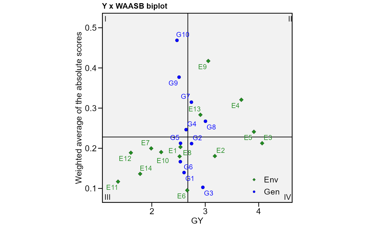
# Plot the scores (response x WAASB)
plot_scores(model3, type = 3)
 # }
# }