![[Stable]](figures/lifecycle-stable.svg)
Compute the Weighted Average of Absolute Scores for AMMI analysis (Olivoto et al., 2019).
This function compute the weighted average of absolute scores, estimated as follows: \[WAAS_i = \sum_{k = 1}^{p} |IPCA_{ik} \times EP_k|/ \sum_{k = 1}^{p}EP_k\]
where \(WAAS_i\) is the weighted average of absolute scores of the
ith genotype; \(IPCA_{ik}\) is the score of the ith genotype
in the kth IPCA; and \(EP_k\) is the explained variance of the kth
IPCA for k = 1,2,..,p, considering p the number of significant
PCAs, or a declared number of PCAs. For example if prob = 0.05, all
axis that are significant considering this probability level are used. The
number of axis can be also informed by declaring naxis = x. This will
override the number of significant axes according to the argument codeprob.
Usage
waas(
  .data,
  env,
  gen,
  rep,
  resp,
  block = NULL,
  mresp = NULL,
  wresp = NULL,
  prob = 0.05,
  naxis = NULL,
  ind_anova = FALSE,
  verbose = TRUE
)
Arguments
- .data
The dataset containing the columns related to Environments, Genotypes, replication/block and response variable(s).
- env
The name of the column that contains the levels of the environments.
- gen
The name of the column that contains the levels of the genotypes.
- rep
The name of the column that contains the levels of the replications/blocks.
- resp
The response variable(s). To analyze multiple variables in a single procedure a vector of variables may be used. For example
resp = c(var1, var2, var3).- block
Defaults to
NULL. In this case, a randomized complete block design is considered. If block is informed, then a resolvable alpha-lattice design (Patterson and Williams, 1976) is employed. All effects, except the error, are assumed to be fixed.- mresp
The new maximum value after rescaling the response variable. By default, all variables in
respare rescaled so that de maximum value is 100 and the minimum value is 0 (i.e.,mresp = NULL). It must be a character vector of the same length ofrespif rescaling is assumed to be different across variables, e.g., if for the first variable smaller values are better and for the second one, higher values are better, thenmresp = c("l, h")must be used. Character value of length 1 will be recycled with a warning message.- wresp
The weight for the response variable(s) for computing the WAASBY index. By default, all variables in
resphave equal weights for mean performance and stability (i.e.,wresp = 50). It must be a numeric vector of the same length ofrespto assign different weights across variables, e.g., if for the first variable equal weights for mean performance and stability are assumed and for the second one, a higher weight for mean performance (e.g. 65) is assumed, thenwresp = c(50, 65)must be used. Numeric value of length 1 will be recycled with a warning message.- prob
The p-value for considering an interaction principal component axis significant.
- naxis
The number of IPCAs to be used for computing the WAAS index. Default is
NULL(Significant IPCAs are used). If values are informed, the number of IPCAS will be used independently on its significance. Note that if two or more variables are included inresp, thennaxismust be a vector.- ind_anova
Logical argument set to
FALSE. IfTRUEan within-environment ANOVA is performed.- verbose
Logical argument. If
verbose = FALSEthe code is run silently.
Value
An object of class waas with the following items for each
variable:
individual A within-environments ANOVA considering a fixed-effect model.
model A data frame with the response variable, the scores of all Principal Components, the estimates of Weighted Average of Absolute Scores, and WAASY (the index that consider the weights for stability and productivity in the genotype ranking.
MeansGxE The means of genotypes in the environments
PCA Principal Component Analysis.
ANOVA Joint analysis of variance for the main effects and Principal Component analysis of the interaction effect.
Details A list summarizing the results. The following information are showed.
WgtResponse, the weight for the response variable in estimating WAASB,WgtWAASthe weight for stability,Ngenthe number of genotypes,Nenvthe number of environments,OVmeanthe overall mean,Minthe minimum observed (returning the genotype and environment),Maxthe maximum observed,Maxthe maximum observed,MinENVthe environment with the lower mean,MaxENVthe environment with the larger mean observed,MinGENthe genotype with the lower mean,MaxGENthe genotype with the larger.augment: Information about each observation in the dataset. This includes predicted values in the
fittedcolumn, residuals in theresidcolumn, standardized residuals in thestdrescolumn, the diagonal of the 'hat' matrix in thehat, and standard errors for the fitted values in these.fitcolumn.probint The p-value for the genotype-vs-environment interaction.
References
Olivoto, T., A.D.C. L\'ucio, J.A.G. da silva, V.S. Marchioro, V.Q. de Souza, and E. Jost. 2019a. Mean performance and stability in multi-environment trials I: Combining features of AMMI and BLUP techniques. Agron. J. 111:2949-2960. doi:10.2134/agronj2019.03.0220
Author
Tiago Olivoto tiagoolivoto@gmail.com
Examples
# \donttest{
library(metan)
#===============================================================#
# Example 1: Analyzing all numeric variables considering p-value#
# <= 0.05 to compute the WAAS. #
#===============================================================#
model <- waas(data_ge,
env = ENV,
gen = GEN,
rep = REP,
resp = everything())
#> variable GY
#> ---------------------------------------------------------------------------
#> AMMI analysis table
#> ---------------------------------------------------------------------------
#> Source Df Sum Sq Mean Sq F value Pr(>F) Proportion Accumulated
#> ENV 13 279.574 21.5057 62.33 0.00e+00 NA NA
#> REP(ENV) 28 9.662 0.3451 3.57 3.59e-08 NA NA
#> GEN 9 12.995 1.4439 14.93 2.19e-19 NA NA
#> GEN:ENV 117 31.220 0.2668 2.76 1.01e-11 NA NA
#> PC1 21 10.749 0.5119 5.29 0.00e+00 34.4 34.4
#> PC2 19 9.924 0.5223 5.40 0.00e+00 31.8 66.2
#> PC3 17 4.039 0.2376 2.46 1.40e-03 12.9 79.2
#> PC4 15 3.074 0.2049 2.12 9.60e-03 9.8 89.0
#> PC5 13 1.446 0.1113 1.15 3.18e-01 4.6 93.6
#> PC6 11 0.932 0.0848 0.88 5.61e-01 3.0 96.6
#> PC7 9 0.567 0.0630 0.65 7.53e-01 1.8 98.4
#> PC8 7 0.362 0.0518 0.54 8.04e-01 1.2 99.6
#> PC9 5 0.126 0.0252 0.26 9.34e-01 0.4 100.0
#> Residuals 252 24.367 0.0967 NA NA NA NA
#> Total 536 389.036 0.7258 NA NA NA NA
#> ---------------------------------------------------------------------------
#>
#> variable HM
#> ---------------------------------------------------------------------------
#> AMMI analysis table
#> ---------------------------------------------------------------------------
#> Source Df Sum Sq Mean Sq F value Pr(>F) Proportion Accumulated
#> ENV 13 5710.32 439.255 57.22 1.11e-16 NA NA
#> REP(ENV) 28 214.93 7.676 2.70 2.20e-05 NA NA
#> GEN 9 269.81 29.979 10.56 7.41e-14 NA NA
#> GEN:ENV 117 1100.73 9.408 3.31 1.06e-15 NA NA
#> PC1 21 381.13 18.149 6.39 0.00e+00 34.6 34.6
#> PC2 19 319.43 16.812 5.92 0.00e+00 29.0 63.6
#> PC3 17 114.26 6.721 2.37 2.10e-03 10.4 74.0
#> PC4 15 81.96 5.464 1.92 2.18e-02 7.4 81.5
#> PC5 13 68.11 5.240 1.84 3.77e-02 6.2 87.7
#> PC6 11 59.07 5.370 1.89 4.10e-02 5.4 93.0
#> PC7 9 46.69 5.188 1.83 6.33e-02 4.2 97.3
#> PC8 7 26.65 3.808 1.34 2.32e-01 2.4 99.7
#> PC9 5 3.41 0.682 0.24 9.45e-01 0.3 100.0
#> Residuals 252 715.69 2.840 NA NA NA NA
#> Total 536 9112.21 17.000 NA NA NA NA
#> ---------------------------------------------------------------------------
#>
#> All variables with significant (p < 0.05) genotype-vs-environment interaction
#> Done!
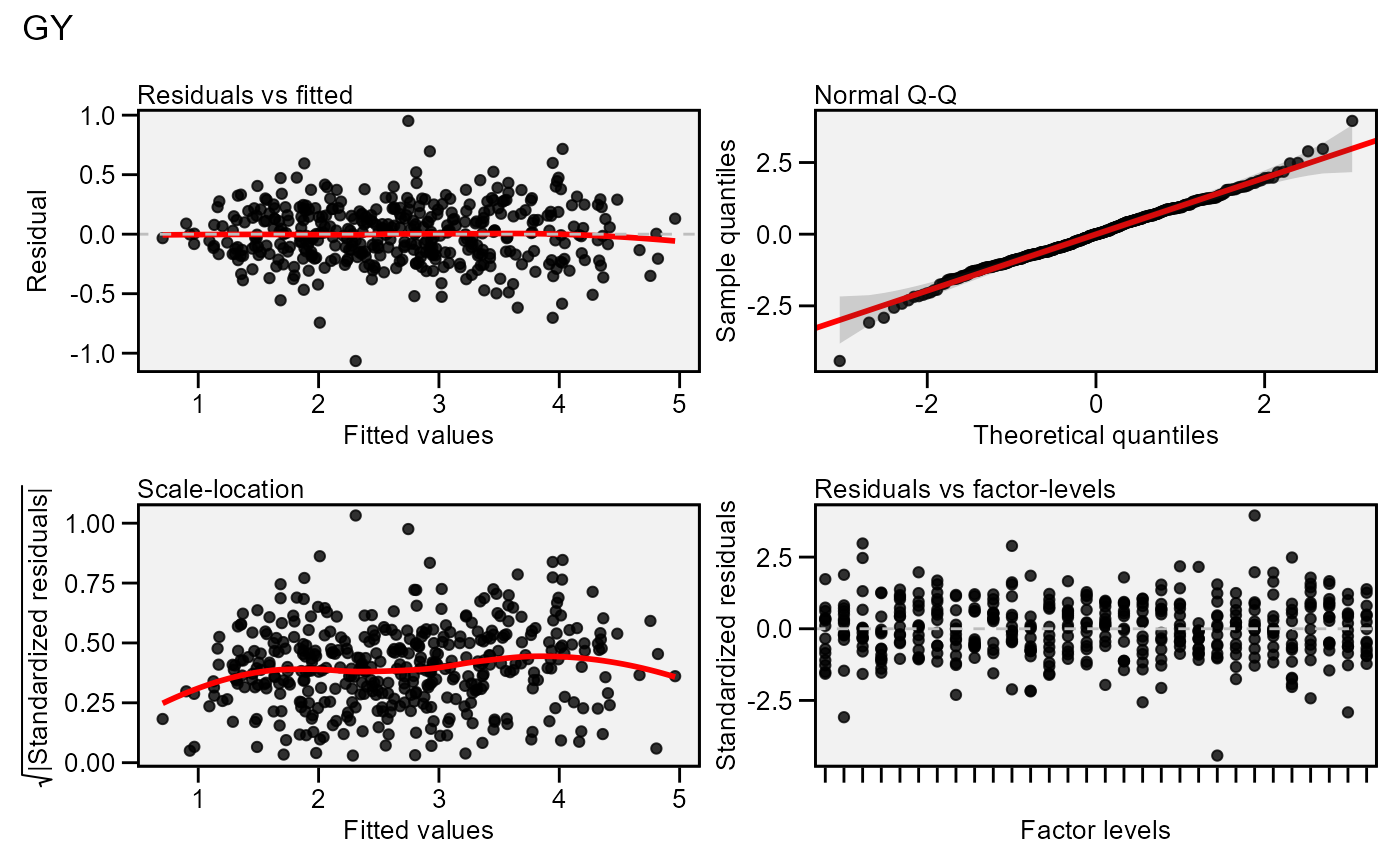
# Residual plot (first variable)
plot(model)
 # Get the WAAS index
get_model_data(model, "WAAS")
#> Class of the model: waas
#> Variable extracted: WAAS
#> # A tibble: 10 × 3
#> GEN GY HM
#> <chr> <dbl> <dbl>
#> 1 G1 0.151 0.455
#> 2 G10 0.652 1.33
#> 3 G2 0.283 0.985
#> 4 G3 0.106 0.418
#> 5 G4 0.326 0.752
#> 6 G5 0.270 1.16
#> 7 G6 0.233 0.478
#> 8 G7 0.428 0.766
#> 9 G8 0.327 0.541
#> 10 G9 0.507 0.701
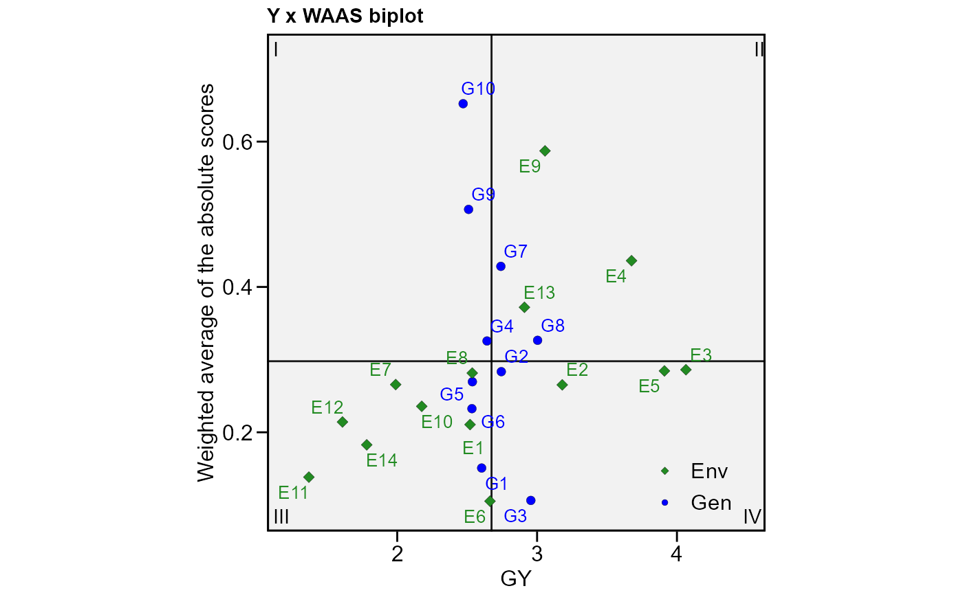
# Plot WAAS and response variable
plot_scores(model, type = 3)
# Get the WAAS index
get_model_data(model, "WAAS")
#> Class of the model: waas
#> Variable extracted: WAAS
#> # A tibble: 10 × 3
#> GEN GY HM
#> <chr> <dbl> <dbl>
#> 1 G1 0.151 0.455
#> 2 G10 0.652 1.33
#> 3 G2 0.283 0.985
#> 4 G3 0.106 0.418
#> 5 G4 0.326 0.752
#> 6 G5 0.270 1.16
#> 7 G6 0.233 0.478
#> 8 G7 0.428 0.766
#> 9 G8 0.327 0.541
#> 10 G9 0.507 0.701
# Plot WAAS and response variable
plot_scores(model, type = 3)
 #===============================================================#
# Example 2: Declaring the number of axis to be used for #
# computing WAAS and assigning a larger weight for the response #
# variable when computing the WAASBY index. #
#===============================================================#
model2 <- waas(data_ge,
env = ENV,
gen = GEN,
rep = REP,
resp = everything(),
naxis = 1, # Only to compare with PC1
wresp = 60)
#> Warning: Invalid length in 'naxis'. Setting naxis = 1 to all the 2 variables.
#> Warning: Invalid length in 'wresp'. Setting wresp = 60 to all the 2 variables.
#> variable GY
#> ---------------------------------------------------------------------------
#> AMMI analysis table
#> ---------------------------------------------------------------------------
#> Source Df Sum Sq Mean Sq F value Pr(>F) Proportion Accumulated
#> ENV 13 279.574 21.5057 62.33 0.00e+00 NA NA
#> REP(ENV) 28 9.662 0.3451 3.57 3.59e-08 NA NA
#> GEN 9 12.995 1.4439 14.93 2.19e-19 NA NA
#> GEN:ENV 117 31.220 0.2668 2.76 1.01e-11 NA NA
#> PC1 21 10.749 0.5119 5.29 0.00e+00 34.4 34.4
#> PC2 19 9.924 0.5223 5.40 0.00e+00 31.8 66.2
#> PC3 17 4.039 0.2376 2.46 1.40e-03 12.9 79.2
#> PC4 15 3.074 0.2049 2.12 9.60e-03 9.8 89.0
#> PC5 13 1.446 0.1113 1.15 3.18e-01 4.6 93.6
#> PC6 11 0.932 0.0848 0.88 5.61e-01 3.0 96.6
#> PC7 9 0.567 0.0630 0.65 7.53e-01 1.8 98.4
#> PC8 7 0.362 0.0518 0.54 8.04e-01 1.2 99.6
#> PC9 5 0.126 0.0252 0.26 9.34e-01 0.4 100.0
#> Residuals 252 24.367 0.0967 NA NA NA NA
#> Total 536 389.036 0.7258 NA NA NA NA
#> ---------------------------------------------------------------------------
#>
#> variable HM
#> ---------------------------------------------------------------------------
#> AMMI analysis table
#> ---------------------------------------------------------------------------
#> Source Df Sum Sq Mean Sq F value Pr(>F) Proportion Accumulated
#> ENV 13 5710.32 439.255 57.22 1.11e-16 NA NA
#> REP(ENV) 28 214.93 7.676 2.70 2.20e-05 NA NA
#> GEN 9 269.81 29.979 10.56 7.41e-14 NA NA
#> GEN:ENV 117 1100.73 9.408 3.31 1.06e-15 NA NA
#> PC1 21 381.13 18.149 6.39 0.00e+00 34.6 34.6
#> PC2 19 319.43 16.812 5.92 0.00e+00 29.0 63.6
#> PC3 17 114.26 6.721 2.37 2.10e-03 10.4 74.0
#> PC4 15 81.96 5.464 1.92 2.18e-02 7.4 81.5
#> PC5 13 68.11 5.240 1.84 3.77e-02 6.2 87.7
#> PC6 11 59.07 5.370 1.89 4.10e-02 5.4 93.0
#> PC7 9 46.69 5.188 1.83 6.33e-02 4.2 97.3
#> PC8 7 26.65 3.808 1.34 2.32e-01 2.4 99.7
#> PC9 5 3.41 0.682 0.24 9.45e-01 0.3 100.0
#> Residuals 252 715.69 2.840 NA NA NA NA
#> Total 536 9112.21 17.000 NA NA NA NA
#> ---------------------------------------------------------------------------
#>
#> All variables with significant (p < 0.05) genotype-vs-environment interaction
#> Done!
# Get the WAAS index (it will be |PC1|)
get_model_data(model2)
#> Class of the model: waas
#> Variable extracted: WAAS
#> # A tibble: 10 × 3
#> GEN GY HM
#> <chr> <dbl> <dbl>
#> 1 G1 0.317 0.280
#> 2 G10 1.00 1.78
#> 3 G2 0.139 1.56
#> 4 G3 0.0434 0.342
#> 5 G4 0.325 0.202
#> 6 G5 0.326 1.58
#> 7 G6 0.0984 0.547
#> 8 G7 0.285 1.22
#> 9 G8 0.499 0.0418
#> 10 G9 0.467 1.07
# Get values for IPCA1
get_model_data(model2, "PC1")
#> Class of the model: waas
#> Variable extracted: PC1
#> # A tibble: 10 × 3
#> GEN GY HM
#> <chr> <dbl> <dbl>
#> 1 G1 0.317 0.280
#> 2 G10 -1.00 -1.78
#> 3 G2 0.139 1.56
#> 4 G3 0.0434 0.342
#> 5 G4 -0.325 -0.202
#> 6 G5 -0.326 1.58
#> 7 G6 -0.0984 0.547
#> 8 G7 0.285 -1.22
#> 9 G8 0.499 -0.0418
#> 10 G9 0.467 -1.07
#===============================================================#
# Example 3: Analyzing GY and HM assuming a random-effect model.#
# Smaller values for HM and higher values for GY are better. #
# To estimate WAASBY, higher weight for the GY (60%) and lower #
# weight for HM (40%) are considered for mean performance. #
#===============================================================#
model3 <- waas(data_ge,
env = ENV,
gen = GEN,
rep = REP,
resp = c(GY, HM),
mresp = c("h, l"),
wresp = c(60, 40))
#> variable GY
#> ---------------------------------------------------------------------------
#> AMMI analysis table
#> ---------------------------------------------------------------------------
#> Source Df Sum Sq Mean Sq F value Pr(>F) Proportion Accumulated
#> ENV 13 279.574 21.5057 62.33 0.00e+00 NA NA
#> REP(ENV) 28 9.662 0.3451 3.57 3.59e-08 NA NA
#> GEN 9 12.995 1.4439 14.93 2.19e-19 NA NA
#> GEN:ENV 117 31.220 0.2668 2.76 1.01e-11 NA NA
#> PC1 21 10.749 0.5119 5.29 0.00e+00 34.4 34.4
#> PC2 19 9.924 0.5223 5.40 0.00e+00 31.8 66.2
#> PC3 17 4.039 0.2376 2.46 1.40e-03 12.9 79.2
#> PC4 15 3.074 0.2049 2.12 9.60e-03 9.8 89.0
#> PC5 13 1.446 0.1113 1.15 3.18e-01 4.6 93.6
#> PC6 11 0.932 0.0848 0.88 5.61e-01 3.0 96.6
#> PC7 9 0.567 0.0630 0.65 7.53e-01 1.8 98.4
#> PC8 7 0.362 0.0518 0.54 8.04e-01 1.2 99.6
#> PC9 5 0.126 0.0252 0.26 9.34e-01 0.4 100.0
#> Residuals 252 24.367 0.0967 NA NA NA NA
#> Total 536 389.036 0.7258 NA NA NA NA
#> ---------------------------------------------------------------------------
#>
#> variable HM
#> ---------------------------------------------------------------------------
#> AMMI analysis table
#> ---------------------------------------------------------------------------
#> Source Df Sum Sq Mean Sq F value Pr(>F) Proportion Accumulated
#> ENV 13 5710.32 439.255 57.22 1.11e-16 NA NA
#> REP(ENV) 28 214.93 7.676 2.70 2.20e-05 NA NA
#> GEN 9 269.81 29.979 10.56 7.41e-14 NA NA
#> GEN:ENV 117 1100.73 9.408 3.31 1.06e-15 NA NA
#> PC1 21 381.13 18.149 6.39 0.00e+00 34.6 34.6
#> PC2 19 319.43 16.812 5.92 0.00e+00 29.0 63.6
#> PC3 17 114.26 6.721 2.37 2.10e-03 10.4 74.0
#> PC4 15 81.96 5.464 1.92 2.18e-02 7.4 81.5
#> PC5 13 68.11 5.240 1.84 3.77e-02 6.2 87.7
#> PC6 11 59.07 5.370 1.89 4.10e-02 5.4 93.0
#> PC7 9 46.69 5.188 1.83 6.33e-02 4.2 97.3
#> PC8 7 26.65 3.808 1.34 2.32e-01 2.4 99.7
#> PC9 5 3.41 0.682 0.24 9.45e-01 0.3 100.0
#> Residuals 252 715.69 2.840 NA NA NA NA
#> Total 536 9112.21 17.000 NA NA NA NA
#> ---------------------------------------------------------------------------
#>
#> All variables with significant (p < 0.05) genotype-vs-environment interaction
#> Done!
# Get the ranks for the WAASY index
get_model_data(model3, what = "OrWAASY")
#> Class of the model: waas
#> Variable extracted: OrWAASY
#> # A tibble: 10 × 3
#> GEN GY HM
#> <chr> <dbl> <dbl>
#> 1 G1 4 1
#> 2 G10 10 9
#> 3 G2 3 4
#> 4 G3 1 2
#> 5 G4 6 7
#> 6 G5 8 10
#> 7 G6 7 3
#> 8 G7 5 6
#> 9 G8 2 8
#> 10 G9 9 5
# }
#===============================================================#
# Example 2: Declaring the number of axis to be used for #
# computing WAAS and assigning a larger weight for the response #
# variable when computing the WAASBY index. #
#===============================================================#
model2 <- waas(data_ge,
env = ENV,
gen = GEN,
rep = REP,
resp = everything(),
naxis = 1, # Only to compare with PC1
wresp = 60)
#> Warning: Invalid length in 'naxis'. Setting naxis = 1 to all the 2 variables.
#> Warning: Invalid length in 'wresp'. Setting wresp = 60 to all the 2 variables.
#> variable GY
#> ---------------------------------------------------------------------------
#> AMMI analysis table
#> ---------------------------------------------------------------------------
#> Source Df Sum Sq Mean Sq F value Pr(>F) Proportion Accumulated
#> ENV 13 279.574 21.5057 62.33 0.00e+00 NA NA
#> REP(ENV) 28 9.662 0.3451 3.57 3.59e-08 NA NA
#> GEN 9 12.995 1.4439 14.93 2.19e-19 NA NA
#> GEN:ENV 117 31.220 0.2668 2.76 1.01e-11 NA NA
#> PC1 21 10.749 0.5119 5.29 0.00e+00 34.4 34.4
#> PC2 19 9.924 0.5223 5.40 0.00e+00 31.8 66.2
#> PC3 17 4.039 0.2376 2.46 1.40e-03 12.9 79.2
#> PC4 15 3.074 0.2049 2.12 9.60e-03 9.8 89.0
#> PC5 13 1.446 0.1113 1.15 3.18e-01 4.6 93.6
#> PC6 11 0.932 0.0848 0.88 5.61e-01 3.0 96.6
#> PC7 9 0.567 0.0630 0.65 7.53e-01 1.8 98.4
#> PC8 7 0.362 0.0518 0.54 8.04e-01 1.2 99.6
#> PC9 5 0.126 0.0252 0.26 9.34e-01 0.4 100.0
#> Residuals 252 24.367 0.0967 NA NA NA NA
#> Total 536 389.036 0.7258 NA NA NA NA
#> ---------------------------------------------------------------------------
#>
#> variable HM
#> ---------------------------------------------------------------------------
#> AMMI analysis table
#> ---------------------------------------------------------------------------
#> Source Df Sum Sq Mean Sq F value Pr(>F) Proportion Accumulated
#> ENV 13 5710.32 439.255 57.22 1.11e-16 NA NA
#> REP(ENV) 28 214.93 7.676 2.70 2.20e-05 NA NA
#> GEN 9 269.81 29.979 10.56 7.41e-14 NA NA
#> GEN:ENV 117 1100.73 9.408 3.31 1.06e-15 NA NA
#> PC1 21 381.13 18.149 6.39 0.00e+00 34.6 34.6
#> PC2 19 319.43 16.812 5.92 0.00e+00 29.0 63.6
#> PC3 17 114.26 6.721 2.37 2.10e-03 10.4 74.0
#> PC4 15 81.96 5.464 1.92 2.18e-02 7.4 81.5
#> PC5 13 68.11 5.240 1.84 3.77e-02 6.2 87.7
#> PC6 11 59.07 5.370 1.89 4.10e-02 5.4 93.0
#> PC7 9 46.69 5.188 1.83 6.33e-02 4.2 97.3
#> PC8 7 26.65 3.808 1.34 2.32e-01 2.4 99.7
#> PC9 5 3.41 0.682 0.24 9.45e-01 0.3 100.0
#> Residuals 252 715.69 2.840 NA NA NA NA
#> Total 536 9112.21 17.000 NA NA NA NA
#> ---------------------------------------------------------------------------
#>
#> All variables with significant (p < 0.05) genotype-vs-environment interaction
#> Done!
# Get the WAAS index (it will be |PC1|)
get_model_data(model2)
#> Class of the model: waas
#> Variable extracted: WAAS
#> # A tibble: 10 × 3
#> GEN GY HM
#> <chr> <dbl> <dbl>
#> 1 G1 0.317 0.280
#> 2 G10 1.00 1.78
#> 3 G2 0.139 1.56
#> 4 G3 0.0434 0.342
#> 5 G4 0.325 0.202
#> 6 G5 0.326 1.58
#> 7 G6 0.0984 0.547
#> 8 G7 0.285 1.22
#> 9 G8 0.499 0.0418
#> 10 G9 0.467 1.07
# Get values for IPCA1
get_model_data(model2, "PC1")
#> Class of the model: waas
#> Variable extracted: PC1
#> # A tibble: 10 × 3
#> GEN GY HM
#> <chr> <dbl> <dbl>
#> 1 G1 0.317 0.280
#> 2 G10 -1.00 -1.78
#> 3 G2 0.139 1.56
#> 4 G3 0.0434 0.342
#> 5 G4 -0.325 -0.202
#> 6 G5 -0.326 1.58
#> 7 G6 -0.0984 0.547
#> 8 G7 0.285 -1.22
#> 9 G8 0.499 -0.0418
#> 10 G9 0.467 -1.07
#===============================================================#
# Example 3: Analyzing GY and HM assuming a random-effect model.#
# Smaller values for HM and higher values for GY are better. #
# To estimate WAASBY, higher weight for the GY (60%) and lower #
# weight for HM (40%) are considered for mean performance. #
#===============================================================#
model3 <- waas(data_ge,
env = ENV,
gen = GEN,
rep = REP,
resp = c(GY, HM),
mresp = c("h, l"),
wresp = c(60, 40))
#> variable GY
#> ---------------------------------------------------------------------------
#> AMMI analysis table
#> ---------------------------------------------------------------------------
#> Source Df Sum Sq Mean Sq F value Pr(>F) Proportion Accumulated
#> ENV 13 279.574 21.5057 62.33 0.00e+00 NA NA
#> REP(ENV) 28 9.662 0.3451 3.57 3.59e-08 NA NA
#> GEN 9 12.995 1.4439 14.93 2.19e-19 NA NA
#> GEN:ENV 117 31.220 0.2668 2.76 1.01e-11 NA NA
#> PC1 21 10.749 0.5119 5.29 0.00e+00 34.4 34.4
#> PC2 19 9.924 0.5223 5.40 0.00e+00 31.8 66.2
#> PC3 17 4.039 0.2376 2.46 1.40e-03 12.9 79.2
#> PC4 15 3.074 0.2049 2.12 9.60e-03 9.8 89.0
#> PC5 13 1.446 0.1113 1.15 3.18e-01 4.6 93.6
#> PC6 11 0.932 0.0848 0.88 5.61e-01 3.0 96.6
#> PC7 9 0.567 0.0630 0.65 7.53e-01 1.8 98.4
#> PC8 7 0.362 0.0518 0.54 8.04e-01 1.2 99.6
#> PC9 5 0.126 0.0252 0.26 9.34e-01 0.4 100.0
#> Residuals 252 24.367 0.0967 NA NA NA NA
#> Total 536 389.036 0.7258 NA NA NA NA
#> ---------------------------------------------------------------------------
#>
#> variable HM
#> ---------------------------------------------------------------------------
#> AMMI analysis table
#> ---------------------------------------------------------------------------
#> Source Df Sum Sq Mean Sq F value Pr(>F) Proportion Accumulated
#> ENV 13 5710.32 439.255 57.22 1.11e-16 NA NA
#> REP(ENV) 28 214.93 7.676 2.70 2.20e-05 NA NA
#> GEN 9 269.81 29.979 10.56 7.41e-14 NA NA
#> GEN:ENV 117 1100.73 9.408 3.31 1.06e-15 NA NA
#> PC1 21 381.13 18.149 6.39 0.00e+00 34.6 34.6
#> PC2 19 319.43 16.812 5.92 0.00e+00 29.0 63.6
#> PC3 17 114.26 6.721 2.37 2.10e-03 10.4 74.0
#> PC4 15 81.96 5.464 1.92 2.18e-02 7.4 81.5
#> PC5 13 68.11 5.240 1.84 3.77e-02 6.2 87.7
#> PC6 11 59.07 5.370 1.89 4.10e-02 5.4 93.0
#> PC7 9 46.69 5.188 1.83 6.33e-02 4.2 97.3
#> PC8 7 26.65 3.808 1.34 2.32e-01 2.4 99.7
#> PC9 5 3.41 0.682 0.24 9.45e-01 0.3 100.0
#> Residuals 252 715.69 2.840 NA NA NA NA
#> Total 536 9112.21 17.000 NA NA NA NA
#> ---------------------------------------------------------------------------
#>
#> All variables with significant (p < 0.05) genotype-vs-environment interaction
#> Done!
# Get the ranks for the WAASY index
get_model_data(model3, what = "OrWAASY")
#> Class of the model: waas
#> Variable extracted: OrWAASY
#> # A tibble: 10 × 3
#> GEN GY HM
#> <chr> <dbl> <dbl>
#> 1 G1 4 1
#> 2 G10 10 9
#> 3 G2 3 4
#> 4 G3 1 2
#> 5 G4 6 7
#> 6 G5 8 10
#> 7 G6 7 3
#> 8 G7 5 6
#> 9 G8 2 8
#> 10 G9 9 5
# }