![[Stable]](figures/lifecycle-stable.svg)
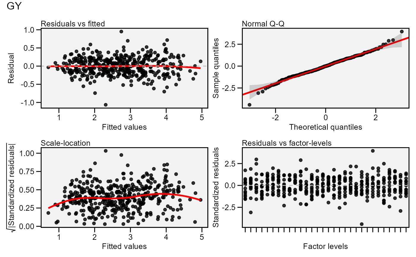
Residual plots for a output model of class performs_ammi,
waas, anova_ind, and anova_joint. Seven types of plots
are produced: (1) Residuals vs fitted, (2) normal Q-Q plot for the residuals,
(3) scale-location plot (standardized residuals vs Fitted Values), (4)
standardized residuals vs Factor-levels, (5) Histogram of raw residuals and
(6) standardized residuals vs observation order, and (7) 1:1 line plot
Usage
residual_plots(
  x,
  var = 1,
  conf = 0.95,
  labels = FALSE,
  plot_theme = theme_metan(),
  band.alpha = 0.2,
  point.alpha = 0.8,
  fill.hist = "gray",
  col.hist = "black",
  col.point = "black",
  col.line = "red",
  col.lab.out = "red",
  size.lab.out = 2.5,
  size.tex.lab = 10,
  size.shape = 1.5,
  bins = 30,
  which = c(1:4),
  ncol = NULL,
  nrow = NULL,
  ...
)
Arguments
- x
An object of class
performs_ammi,waas,anova_joint, orgafem- var
The variable to plot. Defaults to
var = 1the first variable ofx.- conf
Level of confidence interval to use in the Q-Q plot (0.95 by default).
- labels
Logical argument. If
TRUElabels the points outside confidence interval limits.- plot_theme
The graphical theme of the plot. Default is
plot_theme = theme_metan(). For more details, seeggplot2::theme().- band.alpha, point.alpha
The transparency of confidence band in the Q-Q plot and the points, respectively. Must be a number between 0 (opaque) and 1 (full transparency).
- fill.hist
The color to fill the histogram. Default is 'gray'.
- col.hist
The color of the border of the the histogram. Default is 'black'.
- col.point
The color of the points in the graphic. Default is 'black'.
- col.line
The color of the lines in the graphic. Default is 'red'.
- col.lab.out
The color of the labels for the 'outlying' points.
- size.lab.out
The size of the labels for the 'outlying' points.
- size.tex.lab
The size of the text in axis text and labels.
- size.shape
The size of the shape in the plots.
- bins
The number of bins to use in the histogram. Default is 30.
- which
Which graphics should be plotted. Default is
which = c(1:4)that means that the first four graphics will be plotted.- ncol, nrow
The number of columns and rows of the plot pannel. Defaults to
NULL- ...
Additional arguments passed on to the function
patchwork::wrap_plots().
Author
Tiago Olivoto tiagoolivoto@gmail.com
Examples
# \donttest{
library(metan)
model <- performs_ammi(data_ge, ENV, GEN, REP, GY)
#> variable GY
#> ---------------------------------------------------------------------------
#> AMMI analysis table
#> ---------------------------------------------------------------------------
#> Source Df Sum Sq Mean Sq F value Pr(>F) Proportion Accumulated
#> ENV 13 279.574 21.5057 62.33 0.00e+00 NA NA
#> REP(ENV) 28 9.662 0.3451 3.57 3.59e-08 NA NA
#> GEN 9 12.995 1.4439 14.93 2.19e-19 NA NA
#> GEN:ENV 117 31.220 0.2668 2.76 1.01e-11 NA NA
#> PC1 21 10.749 0.5119 5.29 0.00e+00 34.4 34.4
#> PC2 19 9.924 0.5223 5.40 0.00e+00 31.8 66.2
#> PC3 17 4.039 0.2376 2.46 1.40e-03 12.9 79.2
#> PC4 15 3.074 0.2049 2.12 9.60e-03 9.8 89.0
#> PC5 13 1.446 0.1113 1.15 3.18e-01 4.6 93.6
#> PC6 11 0.932 0.0848 0.88 5.61e-01 3.0 96.6
#> PC7 9 0.567 0.0630 0.65 7.53e-01 1.8 98.4
#> PC8 7 0.362 0.0518 0.54 8.04e-01 1.2 99.6
#> PC9 5 0.126 0.0252 0.26 9.34e-01 0.4 100.0
#> Residuals 252 24.367 0.0967 NA NA NA NA
#> Total 536 389.036 0.7258 NA NA NA NA
#> ---------------------------------------------------------------------------
#>
#> All variables with significant (p < 0.05) genotype-vs-environment interaction
#> Done!
# Default plot
plot(model)
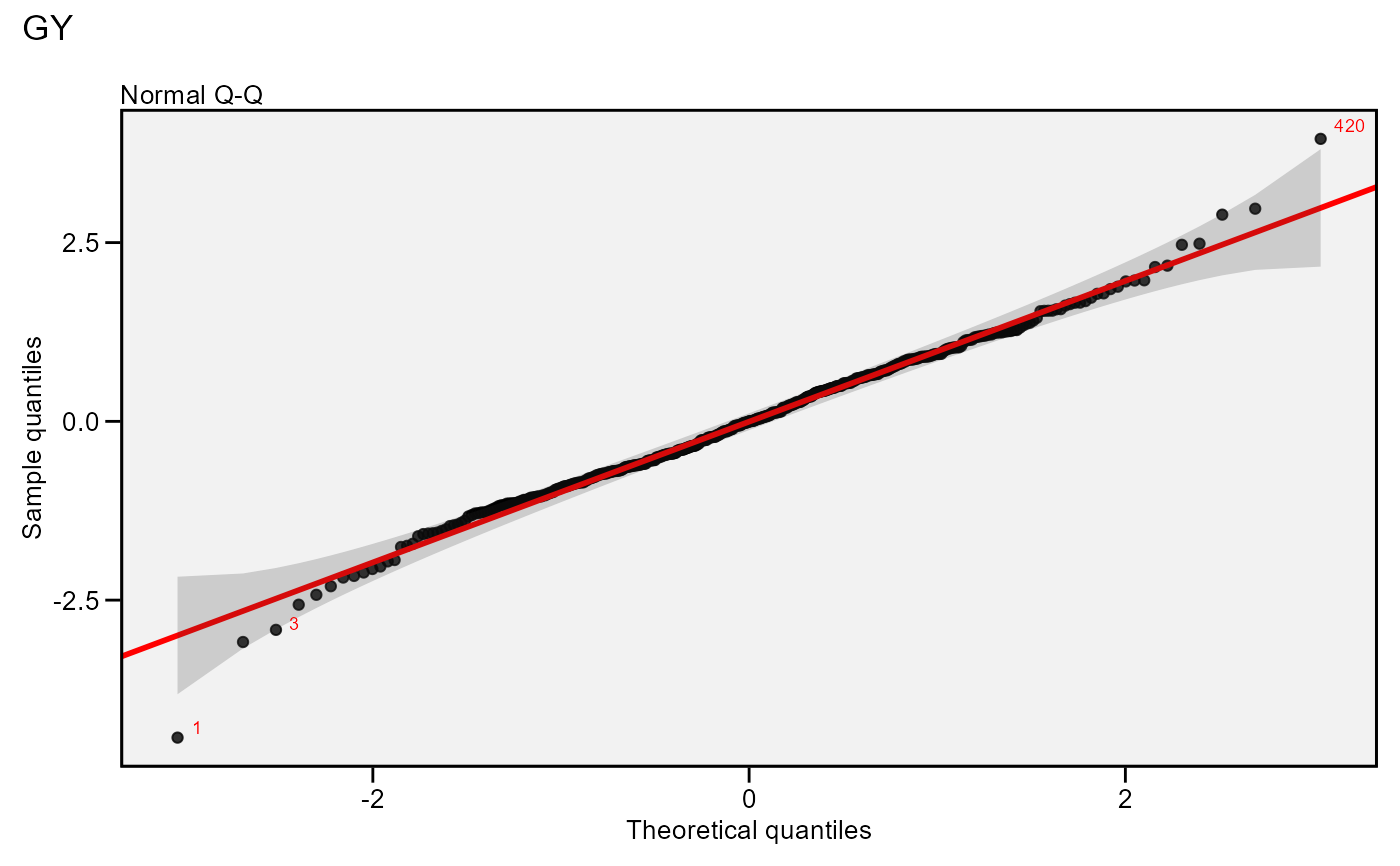
 # Normal Q-Q plot
# Label possible outliers
plot(model,
which = 2,
labels = TRUE)
# Normal Q-Q plot
# Label possible outliers
plot(model,
which = 2,
labels = TRUE)
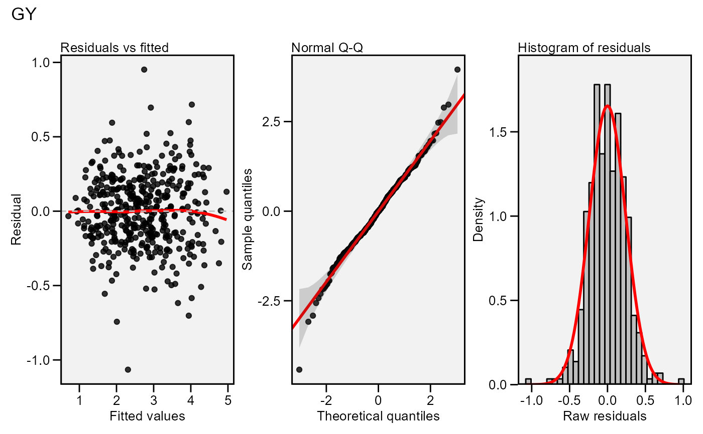
 # Residual vs fitted,
# Normal Q-Q plot
# Histogram of raw residuals
# All in one row
plot(model,
which = c(1, 2, 5),
nrow = 1)
# Residual vs fitted,
# Normal Q-Q plot
# Histogram of raw residuals
# All in one row
plot(model,
which = c(1, 2, 5),
nrow = 1)
 # }
# }