![[Stable]](figures/lifecycle-stable.svg)
Compute the Additive Main effects and Multiplicative interaction (AMMI) model. The estimate of the response variable for the ith genotype in the jth environment (\(y_{ij}\)) using the AMMI model, is given as follows: \[{y_{ij}} = \mu + {\alpha_i} + {\tau_j} + \sum\limits_{k = 1}^p {{\lambda_k}{a_{ik}}} {t_{jk}} + {\rho_{ij}} + {\varepsilon _{ij}}\]
where \(\lambda_k\) is the singular value for the k-th interaction principal component axis (IPCA); \(a_{ik}\) is the i-th element of the k-th eigenvector; \(t_{jk}\) is the jth element of the kth eigenvector. A residual \(\rho _{ij}\) remains, if not all p IPCA are used, where \(p \le min(g - 1; e - 1)\).
This function also serves as a helper function for other procedures performed
in the metan package such as waas() and wsmp()
Arguments
- .data
The dataset containing the columns related to Environments, Genotypes, replication/block and response variable(s).
- env
The name of the column that contains the levels of the environments
- gen
The name of the column that contains the levels of the genotypes
- rep
The name of the column that contains the levels of the replications/blocks
- resp
The response variable(s). To analyze multiple variables in a single procedure, use comma-separated list of unquoted variable names, i.e.,
resp = c(var1, var2, var3), or any select helper likeresp = contains("_PLA").- block
Defaults to
NULL. In this case, a randomized complete block design is considered. If block is informed, then a resolvable alpha-lattice design (Patterson and Williams, 1976) is employed. All effects, except the error, are assumed to be fixed.- verbose
Logical argument. If
verbose = FALSEthe code will run silently.- ...
Arguments passed to the function
impute_missing_val()for imputation of missing values in case of unbalanced data.
Value
ANOVA: The analysis of variance for the AMMI model.
PCA: The principal component analysis
MeansGxE: The means of genotypes in the environments
model: scores for genotypes and environments in all the possible axes.
augment: Information about each observation in the dataset. This includes predicted values in the
fittedcolumn, residuals in theresidcolumn, standardized residuals in thestdrescolumn, the diagonal of the 'hat' matrix in thehat, and standard errors for the fitted values in these.fitcolumn.
References
Patterson, H.D., and E.R. Williams. 1976. A new class of resolvable incomplete block designs. Biometrika 63:83-92.
Author
Tiago Olivoto tiagoolivoto@gmail.com
Examples
# \donttest{
library(metan)
model <- performs_ammi(data_ge, ENV, GEN, REP, resp = c(GY, HM))
#> variable GY
#> ---------------------------------------------------------------------------
#> AMMI analysis table
#> ---------------------------------------------------------------------------
#> Source Df Sum Sq Mean Sq F value Pr(>F) Proportion Accumulated
#> ENV 13 279.574 21.5057 62.33 0.00e+00 NA NA
#> REP(ENV) 28 9.662 0.3451 3.57 3.59e-08 NA NA
#> GEN 9 12.995 1.4439 14.93 2.19e-19 NA NA
#> GEN:ENV 117 31.220 0.2668 2.76 1.01e-11 NA NA
#> PC1 21 10.749 0.5119 5.29 0.00e+00 34.4 34.4
#> PC2 19 9.924 0.5223 5.40 0.00e+00 31.8 66.2
#> PC3 17 4.039 0.2376 2.46 1.40e-03 12.9 79.2
#> PC4 15 3.074 0.2049 2.12 9.60e-03 9.8 89.0
#> PC5 13 1.446 0.1113 1.15 3.18e-01 4.6 93.6
#> PC6 11 0.932 0.0848 0.88 5.61e-01 3.0 96.6
#> PC7 9 0.567 0.0630 0.65 7.53e-01 1.8 98.4
#> PC8 7 0.362 0.0518 0.54 8.04e-01 1.2 99.6
#> PC9 5 0.126 0.0252 0.26 9.34e-01 0.4 100.0
#> Residuals 252 24.367 0.0967 NA NA NA NA
#> Total 536 389.036 0.7258 NA NA NA NA
#> ---------------------------------------------------------------------------
#>
#> variable HM
#> ---------------------------------------------------------------------------
#> AMMI analysis table
#> ---------------------------------------------------------------------------
#> Source Df Sum Sq Mean Sq F value Pr(>F) Proportion Accumulated
#> ENV 13 5710.32 439.255 57.22 1.11e-16 NA NA
#> REP(ENV) 28 214.93 7.676 2.70 2.20e-05 NA NA
#> GEN 9 269.81 29.979 10.56 7.41e-14 NA NA
#> GEN:ENV 117 1100.73 9.408 3.31 1.06e-15 NA NA
#> PC1 21 381.13 18.149 6.39 0.00e+00 34.6 34.6
#> PC2 19 319.43 16.812 5.92 0.00e+00 29.0 63.6
#> PC3 17 114.26 6.721 2.37 2.10e-03 10.4 74.0
#> PC4 15 81.96 5.464 1.92 2.18e-02 7.4 81.5
#> PC5 13 68.11 5.240 1.84 3.77e-02 6.2 87.7
#> PC6 11 59.07 5.370 1.89 4.10e-02 5.4 93.0
#> PC7 9 46.69 5.188 1.83 6.33e-02 4.2 97.3
#> PC8 7 26.65 3.808 1.34 2.32e-01 2.4 99.7
#> PC9 5 3.41 0.682 0.24 9.45e-01 0.3 100.0
#> Residuals 252 715.69 2.840 NA NA NA NA
#> Total 536 9112.21 17.000 NA NA NA NA
#> ---------------------------------------------------------------------------
#>
#> All variables with significant (p < 0.05) genotype-vs-environment interaction
#> Done!
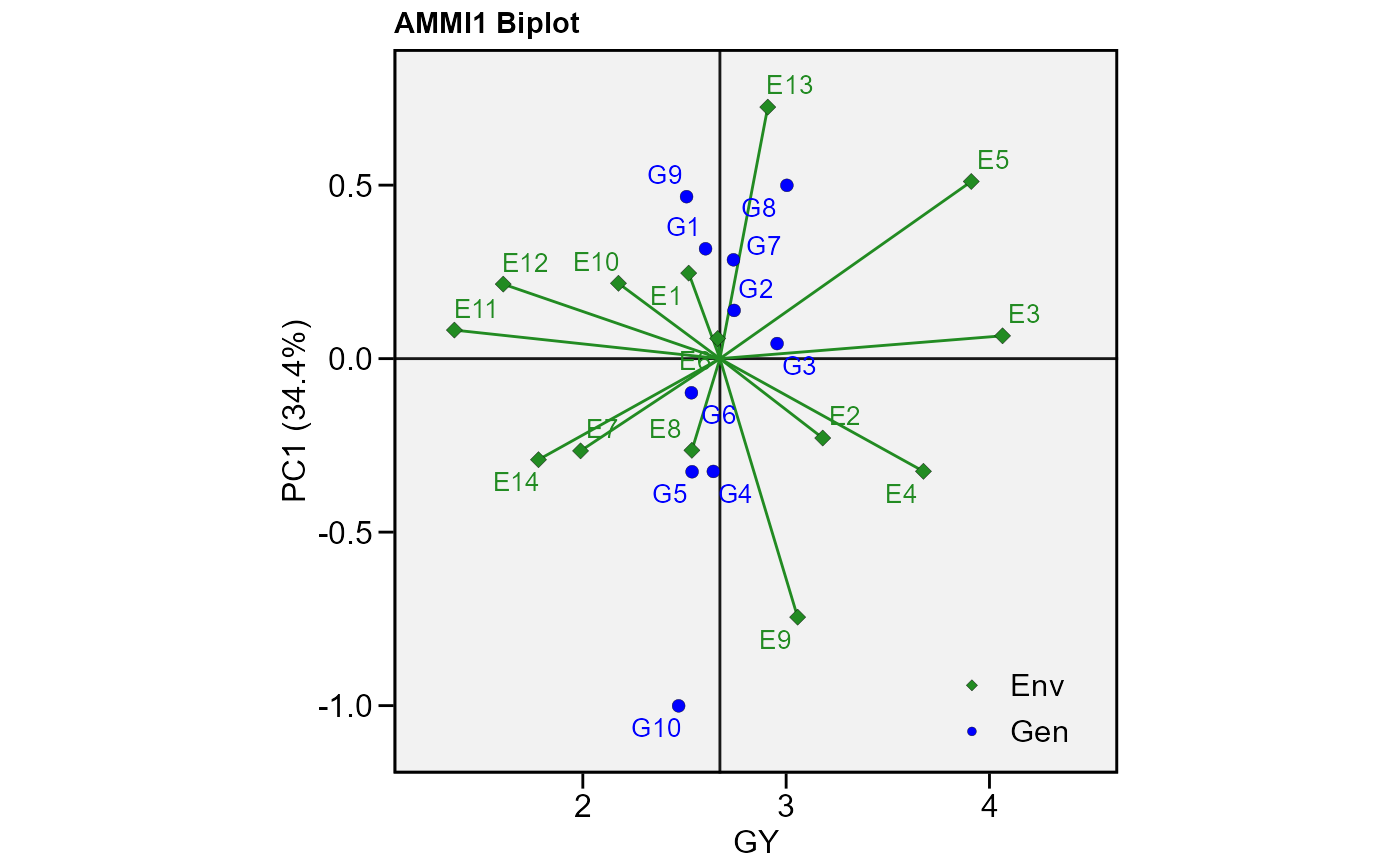
# PC1 x PC2 (variable GY)
p1 <- plot_scores(model)
p1
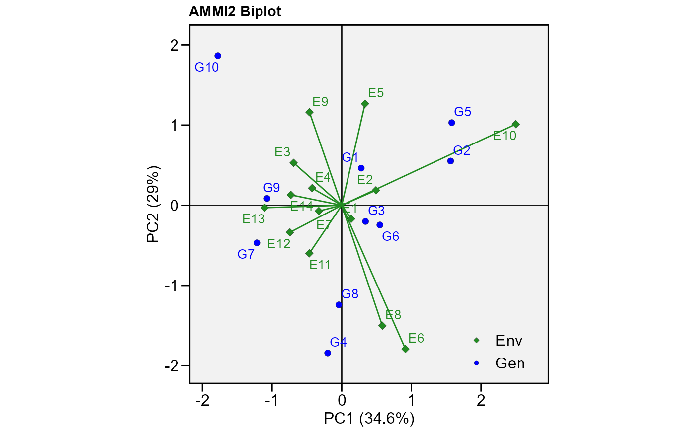
 # PC1 x PC2 (variable HM)
plot_scores(model,
var = 2, # or "HM"
type = 2)
# PC1 x PC2 (variable HM)
plot_scores(model,
var = 2, # or "HM"
type = 2)
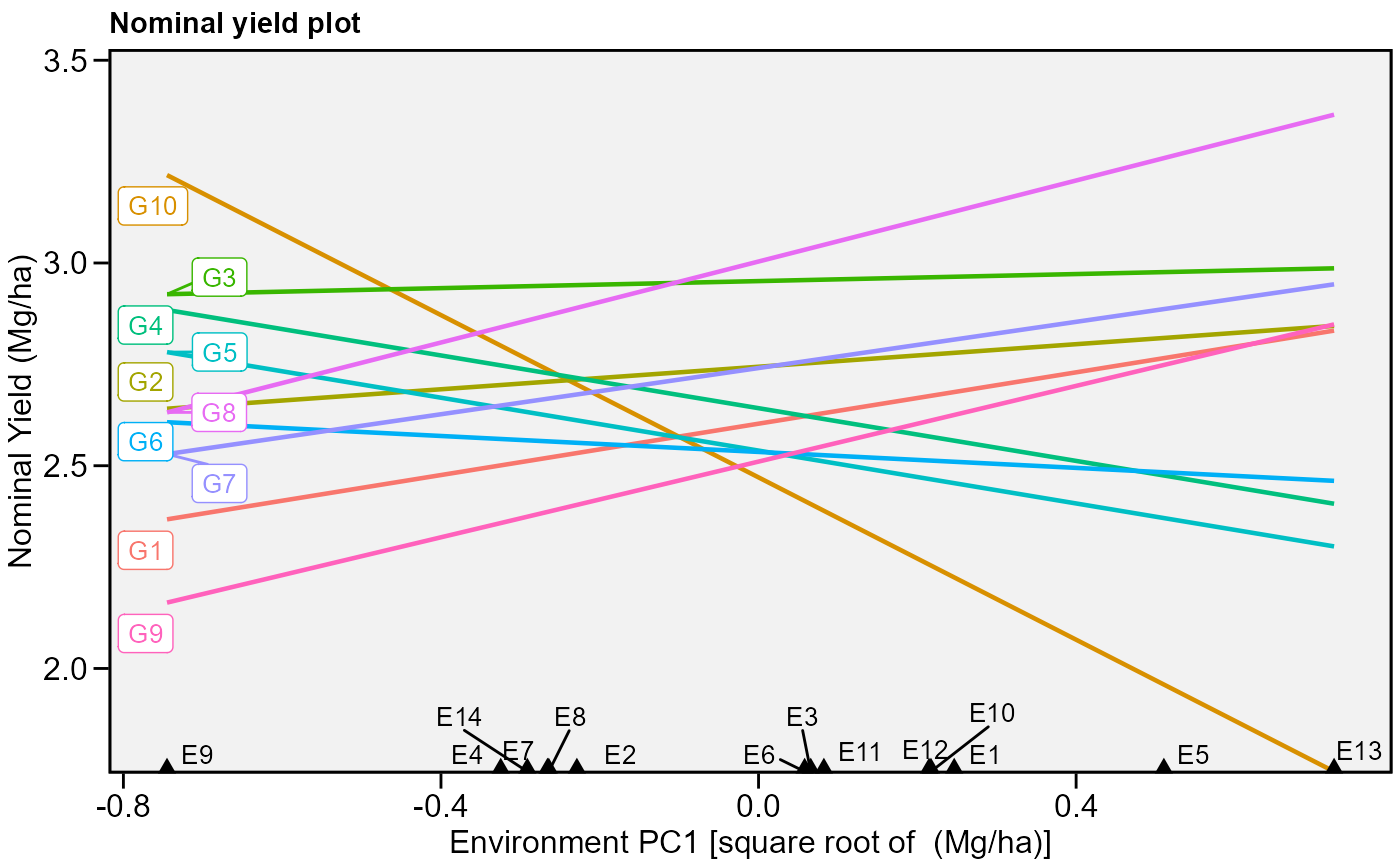
 # Nominal yield plot (variable GY)
# Draw a convex hull polygon
plot_scores(model, type = 4)
# Nominal yield plot (variable GY)
# Draw a convex hull polygon
plot_scores(model, type = 4)
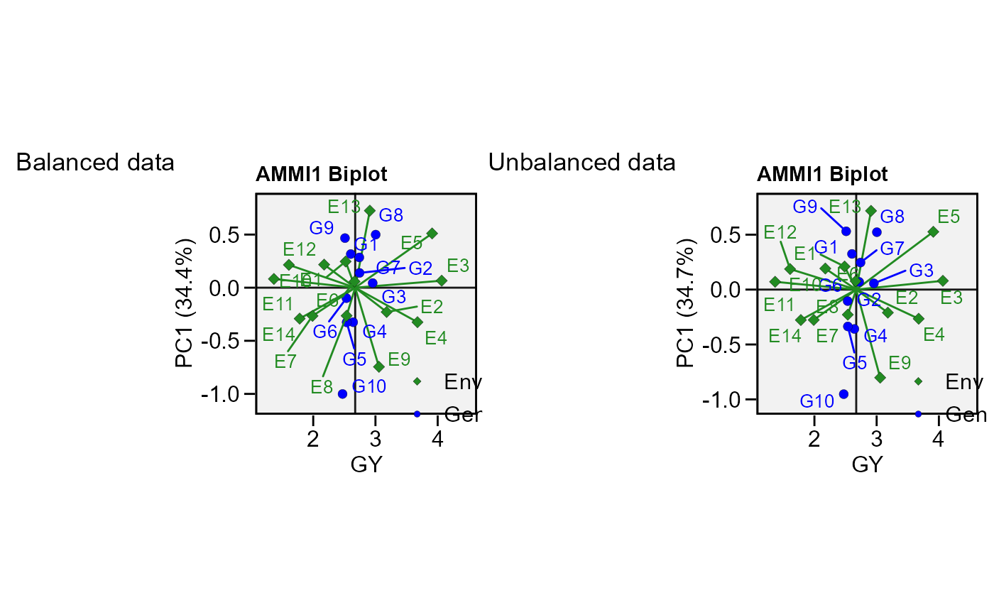
 # Unbalanced data (GEN 2 in E1 missing)
mod <-
data_ge %>%
remove_rows(4:6) %>%
droplevels() %>%
performs_ammi(ENV, GEN, REP, GY)
#> ----------------------------------------------
#> Convergence information
#> ----------------------------------------------
#> Number of iterations: 13
#> Final RMSE: 6.836709e-11
#> Number of axis: 1
#> Convergence: TRUE
#> ----------------------------------------------
#> Warning: Data imputation used to fill the GxE matrix
#> variable GY
#> ---------------------------------------------------------------------------
#> AMMI analysis table
#> ---------------------------------------------------------------------------
#> Source Df Sum Sq Mean Sq F value Pr(>F) Proportion Accumulated
#> ENV 13 279.841 21.5262 62.86 0.00e+00 NA NA
#> REP(ENV) 28 9.589 0.3425 3.53 4.80e-08 NA NA
#> GEN 9 12.919 1.4354 14.81 3.31e-19 NA NA
#> GEN:ENV 116 30.872 0.2661 2.75 1.53e-11 NA NA
#> PC1 21 10.699 0.5095 5.26 0.00e+00 34.7 34.7
#> PC2 19 9.853 0.5186 5.35 0.00e+00 31.9 66.6
#> PC3 17 3.844 0.2261 2.33 2.60e-03 12.5 79.0
#> PC4 15 3.044 0.2029 2.09 1.09e-02 9.9 88.9
#> PC5 13 1.439 0.1107 1.14 3.26e-01 4.7 93.5
#> PC6 11 0.891 0.0810 0.84 6.00e-01 2.9 96.4
#> PC7 9 0.590 0.0656 0.68 7.27e-01 1.9 98.3
#> PC8 7 0.389 0.0556 0.57 7.80e-01 1.3 99.6
#> PC9 5 0.122 0.0244 0.25 9.40e-01 0.4 100.0
#> Residuals 250 24.231 0.0969 NA NA NA NA
#> Total 533 388.325 0.7286 NA NA NA NA
#> ---------------------------------------------------------------------------
#>
#> All variables with significant (p < 0.05) genotype-vs-environment interaction
#> Done!
p2 <- plot_scores(mod)
arrange_ggplot(p1, p2, tag_levels = list(c("Balanced data", "Unbalanced data")))
# Unbalanced data (GEN 2 in E1 missing)
mod <-
data_ge %>%
remove_rows(4:6) %>%
droplevels() %>%
performs_ammi(ENV, GEN, REP, GY)
#> ----------------------------------------------
#> Convergence information
#> ----------------------------------------------
#> Number of iterations: 13
#> Final RMSE: 6.836709e-11
#> Number of axis: 1
#> Convergence: TRUE
#> ----------------------------------------------
#> Warning: Data imputation used to fill the GxE matrix
#> variable GY
#> ---------------------------------------------------------------------------
#> AMMI analysis table
#> ---------------------------------------------------------------------------
#> Source Df Sum Sq Mean Sq F value Pr(>F) Proportion Accumulated
#> ENV 13 279.841 21.5262 62.86 0.00e+00 NA NA
#> REP(ENV) 28 9.589 0.3425 3.53 4.80e-08 NA NA
#> GEN 9 12.919 1.4354 14.81 3.31e-19 NA NA
#> GEN:ENV 116 30.872 0.2661 2.75 1.53e-11 NA NA
#> PC1 21 10.699 0.5095 5.26 0.00e+00 34.7 34.7
#> PC2 19 9.853 0.5186 5.35 0.00e+00 31.9 66.6
#> PC3 17 3.844 0.2261 2.33 2.60e-03 12.5 79.0
#> PC4 15 3.044 0.2029 2.09 1.09e-02 9.9 88.9
#> PC5 13 1.439 0.1107 1.14 3.26e-01 4.7 93.5
#> PC6 11 0.891 0.0810 0.84 6.00e-01 2.9 96.4
#> PC7 9 0.590 0.0656 0.68 7.27e-01 1.9 98.3
#> PC8 7 0.389 0.0556 0.57 7.80e-01 1.3 99.6
#> PC9 5 0.122 0.0244 0.25 9.40e-01 0.4 100.0
#> Residuals 250 24.231 0.0969 NA NA NA NA
#> Total 533 388.325 0.7286 NA NA NA NA
#> ---------------------------------------------------------------------------
#>
#> All variables with significant (p < 0.05) genotype-vs-environment interaction
#> Done!
p2 <- plot_scores(mod)
arrange_ggplot(p1, p2, tag_levels = list(c("Balanced data", "Unbalanced data")))
 # }
# }