Left-aligned y tick labels

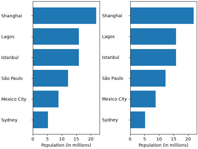
By default, tick labels are aligned towards the axis. This means the set of y tick labels appear right-aligned.

To obtain left-aligned y tick labels, a solution is to force their horizontal-alignment to "left". However, because the alignment reference point is on the axis, such labels would overlap the plotting area, so the label padding needs to be additionally increased.

An alternate solution is to use the mathtext commands \rlap and \phantom to manipulate the widths of the tick labels as seen by Matplotlib. See https://www.tug.org/TUGboat/tb22-4/tb72perlS.pdf for a detailed description of this approach.

See also Ticklabel alignment.

import matplotlib.pyplot as plt

population = {
    "Sydney": 5.2,
    "Mexico City": 8.8,
    "São Paulo": 12.2,
    "Istanbul": 15.9,
    "Lagos": 15.9,
    "Shanghai": 21.9,
}

fig, axs = plt.subplots(1, 2, layout="constrained")

# First solution: Force the horizontal-alignment of y tick labels to "left",
# and increase the padding (to a manually chosen value).

ax = axs[0]
ax.barh(population.keys(), population.values())
ax.set_xlabel('Population (in millions)')
for ticklabel in ax.get_yticklabels():
    ticklabel.set_horizontalalignment("left")
ax.tick_params("y", pad=70)


# Second solution: Use mathtext to manipulate the width of ylabels as seen
# by Matplotlib.  Here, \rlap means "draw this text, but don't advance the
# cursor", whereas \phantom means "advance the cursor by the width of the
# enclosed text, but without actually drawing the text".  The end result is
# that the labels get aligned as if "Mexico City" was written every time, but
# the real labels are actually drawn.

# Note that the widest label ("Mexico City") is still hard-coded here (it is
# the widest *rendered* label, which is not necessarily the longest label in
# characters).
def left_aligned_label(s):
    return r"$\rlap{\text{%s}}\phantom{\text{Mexico City}}$" % s

ax = axs[1]
ax.barh([*map(left_aligned_label, population)], population.values())
ax.set_xlabel('Population (in millions)')

plt.show()