Support Vector Machines (SVMs)- Supervised Image Classification
Support Vector Machines (SVMs) are supervised learning algorithms used mostly for classification problems. SVM models apply non-linear functions to select the best relationship between the response variable and predictors by introducing kernels functions that map the independent variables to higher dimensional feature spaces . This approach typically leads to a better generalization of the chosen model on out-of-sample data . The principle behind an SVM classifier algorithm is to separate data into different classes using a hyperplane. The goal in choosing a hyperplane is to maximize the distance from the hyperplane to the nearest data point of either class . These nearest data points are known as Support Vectors.
Load R packages
library(caret)        # machine laerning
library(kernlab)      # support vector machine
library(rgdal)        # spatial data processing
library(raster)       # raster processing
library(plyr)         # data manipulation
library(dplyr)        # data manipulation
library(RStoolbox)    # ploting spatial data
library(RColorBrewer) # color
library(ggplot2)      # ploting
library(sp)           # spatial data
library(doParallel)   # Parallel processing
The data could be available for download from here.
# Define data folder
dataFolder<-"F://Spatial_Data_Processing_and_Analysis_R//Data//DATA_09//"
Load data
train.df<-read.csv(paste0(dataFolder,".\\Sentinel_2\\train_data.csv"), header = T)
test.df<-read.csv(paste0(dataFolder,".\\Sentinel_2\\test_data.csv"), header = T)
Start foreach to parallelize for model fitting
mc <- makeCluster(detectCores())
registerDoParallel(mc)
Tunning prameters
myControl <- trainControl(method="repeatedcv",
                          number=3,
                          repeats=2,
                          returnResamp='all',
                          allowParallel=TRUE)
Train SVM model
We will use the train() function from the caret package with “method” parameter “svmRadial” (Radial Based Kernel based classification) wrapped from the Kernlab package.
set.seed(849)
fit.svm <- train(as.factor(Landuse)~B2+B3+B4+B4+B6+B7+B8+B8A+B11+B12,
                data=train.df,
                method = "svmRadial",
                metric= "Accuracy",
                preProc = c("center", "scale"),
                trControl = myControl
                )
fit.svm
## Support Vector Machines with Radial Basis Function Kernel
##
## 16764 samples
## 9 predictor
## 5 classes: 'Building', 'Grass', 'Parking/road/pavement', 'Tree/bushes', 'Water'
##
## Pre-processing: centered (9), scaled (9)
## Resampling: Cross-Validated (3 fold, repeated 2 times)
## Summary of sample sizes: 11176, 11175, 11177, 11175, 11175, 11178, ...
## Resampling results across tuning parameters:
##
## C Accuracy Kappa
## 0.25 0.9589598 0.9455614
## 0.50 0.9672515 0.9565454
## 1.00 0.9769151 0.9693513
##
## Tuning parameter 'sigma' was held constant at a value of 1.526924
## Accuracy was used to select the optimal model using the largest value.
## The final values used for the model were sigma = 1.526924 and C = 1.Stop cluster
stopCluster(mc)Confusion Matrix - train data
p1<-predict(fit.svm, train.df, type = "raw")
confusionMatrix(p1, train.df$Landuse)
## Confusion Matrix and Statistics
##
## Reference
## Prediction Building Grass Parking/road/pavement Tree/bushes
## Building 2990 0 52 0
## Grass 0 3437 0 8
## Parking/road/pavement 70 0 3810 58
## Tree/bushes 41 45 12 5602
## Water 0 0 0 0
## Reference
## Prediction Water
## Building 0
## Grass 0
## Parking/road/pavement 0
## Tree/bushes 11
## Water 628
##
## Overall Statistics
##
## Accuracy : 0.9823
## 95% CI : (0.9802, 0.9842)
## No Information Rate : 0.3381
## P-Value [Acc > NIR] : < 2.2e-16
##
## Kappa : 0.9765
## Mcnemar's Test P-Value : NA
##
## Statistics by Class:
##
## Class: Building Class: Grass
## Sensitivity 0.9642 0.9871
## Specificity 0.9962 0.9994
## Pos Pred Value 0.9829 0.9977
## Neg Pred Value 0.9919 0.9966
## Prevalence 0.1850 0.2077
## Detection Rate 0.1784 0.2050
## Detection Prevalence 0.1815 0.2055
## Balanced Accuracy 0.9802 0.9932
## Class: Parking/road/pavement Class: Tree/bushes
## Sensitivity 0.9835 0.9884
## Specificity 0.9901 0.9902
## Pos Pred Value 0.9675 0.9809
## Neg Pred Value 0.9950 0.9940
## Prevalence 0.2311 0.3381
## Detection Rate 0.2273 0.3342
## Detection Prevalence 0.2349 0.3407
## Balanced Accuracy 0.9868 0.9893
## Class: Water
## Sensitivity 0.98279
## Specificity 1.00000
## Pos Pred Value 1.00000
## Neg Pred Value 0.99932
## Prevalence 0.03812
## Detection Rate 0.03746
## Detection Prevalence 0.03746
## Balanced Accuracy 0.99139Confusion Matrix - test data
p2<-predict(fit.svm, test.df, type = "raw")
confusionMatrix(p2, test.df$Landuse)
## Confusion Matrix and Statistics
##
## Reference
## Prediction Building Grass Parking/road/pavement Tree/bushes
## Building 1278 0 30 0
## Grass 0 1472 0 5
## Parking/road/pavement 34 0 1625 23
## Tree/bushes 16 19 5 2401
## Water 0 0 0 0
## Reference
## Prediction Water
## Building 0
## Grass 0
## Parking/road/pavement 0
## Tree/bushes 7
## Water 266
##
## Overall Statistics
##
## Accuracy : 0.9806
## 95% CI : (0.9772, 0.9837)
## No Information Rate : 0.3383
## P-Value [Acc > NIR] : < 2.2e-16
##
## Kappa : 0.9743
## Mcnemar's Test P-Value : NA
##
## Statistics by Class:
##
## Class: Building Class: Grass
## Sensitivity 0.9623 0.9873
## Specificity 0.9949 0.9991
## Pos Pred Value 0.9771 0.9966
## Neg Pred Value 0.9915 0.9967
## Prevalence 0.1849 0.2076
## Detection Rate 0.1780 0.2050
## Detection Prevalence 0.1821 0.2057
## Balanced Accuracy 0.9786 0.9932
## Class: Parking/road/pavement Class: Tree/bushes
## Sensitivity 0.9789 0.9885
## Specificity 0.9897 0.9901
## Pos Pred Value 0.9661 0.9808
## Neg Pred Value 0.9936 0.9941
## Prevalence 0.2312 0.3383
## Detection Rate 0.2263 0.3344
## Detection Prevalence 0.2342 0.3409
## Balanced Accuracy 0.9843 0.9893
## Class: Water
## Sensitivity 0.97436
## Specificity 1.00000
## Pos Pred Value 1.00000
## Neg Pred Value 0.99899
## Prevalence 0.03802
## Detection Rate 0.03704
## Detection Prevalence 0.03704
## Balanced Accuracy 0.98718Predition at grid location
# read grid CSV file
grid.df<-read.csv(paste0(dataFolder,".\\Sentinel_2\\prediction_grid_data.csv"), header = T)
# Preddict at grid location
p3<-as.data.frame(predict(fit.svm, grid.df, type = "raw"))
# Extract predicted landuse class
grid.df$Landuse<-p3$predict
# Import lnaduse ID file
ID<-read.csv(paste0(dataFolder,".\\Sentinel_2\\Landuse_ID.csv"), header=T)
# Join landuse ID
grid.new<-join(grid.df, ID, by="Landuse", type="inner")
# Omit missing values
grid.new.na<-na.omit(grid.new)
Convert to raster
x<-SpatialPointsDataFrame(as.data.frame(grid.new.na)[, c("x", "y")], data = grid.new.na)
r <- rasterFromXYZ(as.data.frame(x)[, c("x", "y", "Class_ID")])
Plot Landuse Map:
# Color Palette
myPalette <- colorRampPalette(c("light grey","burlywood4", "forestgreen","light green", "dodgerblue"))
# Plot Map
LU<-spplot(r,"Class_ID", main="Supervised Image Classification: svmRadial" ,
      colorkey = list(space="right",tick.number=1,height=1, width=1.5,
              labels = list(at = seq(1,4.8,length=5),cex=1.0,
              lab = c("Road/parking/pavement" ,"Building", "Tree/buses", "Grass", "Water"))),
              col.regions=myPalette,cut=4)
LU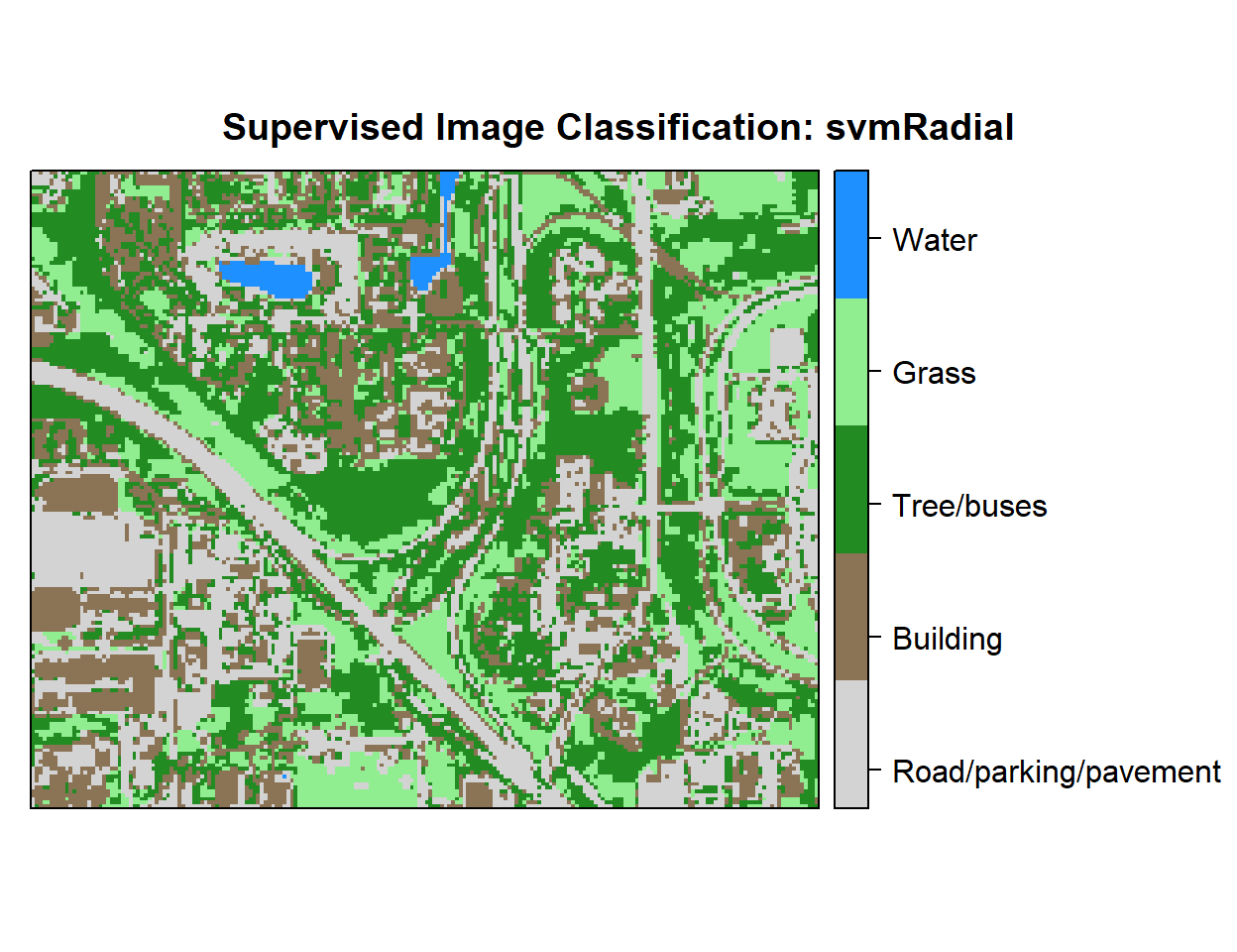
Write raster
# writeRaster(r, filename = paste0(dataFolder,".\\Sentinel_2\\SVM_Landuse.tiff"), "GTiff", overwrite=T)rm(list = ls())