Export Plots in R: ggsave, Devices, DPI and Journal Specs
A plot on your screen is temporary. To put it in a report, a slide deck, or a journal submission you have to write it to a file, and in R the one function that does this is ggsave(). You give it a name, a size, and a resolution, and it picks the right file format from the extension. Everything else in this tutorial, from graphics devices to DPI to journal specs, is detail layered on top of that one call. You only need the ggplot2 package throughout.
How do you save a plot in R with ggsave()?
You have built a plot you like. Now a colleague asks for "the image", or a journal wants a figure file, and taking a screenshot gives you a blurry, wrong-sized picture. The proper fix is to render the plot straight to a file at the exact size and sharpness you want, and ggsave() is the tool for that.
Let's make a plot first so we have something to save. We will load ggplot2, build a simple scatter plot of car weight against fuel economy using the built-in mtcars data, and store it in an object called p. Storing the plot in a variable matters, because ggsave() can then save that exact object rather than guessing what was last on screen.
That is the whole idea in one block. We built p, chose a file path (here inside R's temporary folder so nothing clutters your project), and called ggsave() with a width and height in inches plus a 300 DPI resolution. The file.exists() check returns TRUE, which confirms a real PNG image now sits on disk. Notice we never wrote the word "PNG" anywhere except in the file name: ggsave() read the .png extension and chose the PNG format for us.
plot.png and you get a PNG, name it plot.pdf and you get a PDF, with no extra argument needed. That one rule is why ggsave() feels so simple: the extension alone decides the format. For a deeper reference on every argument, see the ggsave() guide.Try it: Save the same plot p as a JPEG instead of a PNG. All you need to change is the file extension in the path.
Click to reveal solution
Explanation: Changing .png to .jpeg is all it takes. ggsave() sees the new extension and writes a JPEG. We dropped the dpi argument here, so it uses the default of 300.
What do width, height, and units control?
Width and height set the physical size of the saved figure, not the number of pixels directly. Think of it as the size the figure would be if you printed it and held a ruler to it. By default ggsave() reads those two numbers as inches, so width = 6, height = 4 means a six-inch by four-inch figure.
You are not stuck with inches. The units argument accepts "in", "cm", "mm", or "px", so you can speak in whatever the situation calls for. Journals usually quote sizes in millimetres, screens in pixels, and everyday work in inches or centimetres. Let's save the plot at 16 centimetres wide by 10 centimetres tall, then confirm how big that is in inches so the two systems feel connected.
The file saved cleanly, and the arithmetic shows that 16 cm is about 6.3 inches, so this figure is close in size to the six-inch version from the first section. That is the point of units: it changes the label on the number, not the way ggsave() works. Pick whichever unit matches the spec you were handed and let R do the conversion.
ggsave() falls back to the current on-screen plotting size, which varies with your window and gives you a different figure every time. Naming an explicit width and height makes the output reproducible, so the file looks the same on any machine.Try it: Save p at 12 cm wide and 8 cm tall. Reuse the units = "cm" argument.
Click to reveal solution
Explanation: With units = "cm", the numbers 12 and 8 are read as centimetres. The saved file is a smaller version of the same plot.
What is DPI and how does it set image resolution?
DPI stands for dots per inch, and it is the bridge between physical size and pixel count. A raster image (one made of a grid of coloured dots) needs to know how many dots to pack into each inch. More dots per inch means a sharper image, because fine details have more pixels to live in. The relationship is simple multiplication: the number of pixels along a side equals the size in inches times the DPI.
Let's make that concrete. A figure six inches wide at 300 DPI is 1800 pixels across, and four inches tall is 1200 pixels down. We will compute both numbers so you can see the rule in action rather than just read it.
So a six-by-four-inch figure at 300 DPI is an 1800 by 1200 pixel image. If you had asked for 72 DPI, the same physical figure would be only 432 by 288 pixels, which is why low-DPI exports look soft when you zoom in: there simply are not enough dots. To see the effect on the file itself, let's save the same plot at a low DPI and a high DPI and compare the file sizes.
The 300 DPI file is larger because it stores far more pixels for the same six-by-four-inch area. That is the trade-off in a nutshell: higher DPI gives you a crisper image and a bigger file. For quick web previews, 72 or 96 DPI is fine; for anything printed, 300 is the usual floor. ggsave() even accepts the shortcuts dpi = "screen" (72), dpi = "print" (300), and dpi = "retina" (320) if you prefer names to numbers.
Try it: Work out how many pixels wide an eight-inch figure would be at 600 DPI. Fix the DPI in the multiplication below.
Click to reveal solution
Explanation: Pixels equal inches times DPI, so 8 inches at 600 DPI is 4800 pixels wide. That is the kind of resolution a journal asks for in high-quality line art.
Which file format should you export: PNG, JPEG, TIFF, PDF, or SVG?
Every format falls into one of two families, and knowing which family you need answers most of the question. Raster formats store the image as a grid of pixels, so they have a fixed resolution and can blur when enlarged past their DPI. Vector formats store the image as instructions ("draw a line here, a circle there"), so they redraw perfectly at any size. Here is how the common formats compare.
| Format | Type | Best for | Notes |
|---|---|---|---|
| PNG | Raster | Web, slides, reports | Lossless and sharp, small files for plots |
| JPEG | Raster | Photographs | Lossy, blurs text and thin lines |
| TIFF | Raster | Print and journals | Lossless, large, a print standard |
| Vector | Print, LaTeX, scaling | Stays sharp at any size | |
| SVG | Vector | Web and editing | Editable later in design tools |
The flow below turns that table into a quick decision you can make in a second.
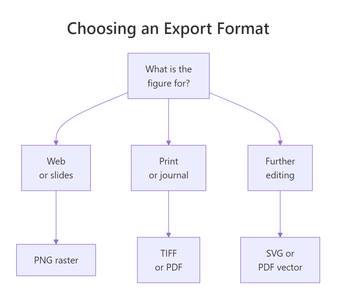
Figure 1: A quick way to pick a file format from what the figure is for.
Because ggsave() reads the extension, switching formats is just switching the ending on the filename. Let's save p in four formats at once by looping over a list of extensions, then confirm every file was written.
All four files exist, each written by the device that matches its extension. The PNG and JPEG are pixel grids, the TIFF is a high-quality pixel grid built for print, and the PDF is a vector file you can drop into a document or a LaTeX report without ever losing sharpness.
SVG is the one common format that needs a helper package. Modern ggplot2 exports SVG through the svglite package, which is not part of the in-browser toolset used on this page, so the block below is written to run locally in your own RStudio session rather than here.
# Run this in RStudio: SVG export needs the svglite package
library(svglite)
library(ggplot2)

svg_file <- file.path(tempdir(), "fuel.svg")
ggsave(svg_file, plot = p, width = 6, height = 4)  # ggsave uses svglite for .svg
file.exists(svg_file)
#> [1] TRUE
Once svglite is installed, ggsave("plot.svg", ...) works exactly like the other formats. The result is a fully editable vector file you can open in Inkscape or Illustrator to tweak labels by hand before publication.
Try it: Save p as a vector PDF called report-fig.pdf. Vectors stay sharp when a reader zooms in, which is ideal for documents.
Click to reveal solution
Explanation: The .pdf extension tells ggsave() to use the PDF device, producing a vector file that prints crisply at any size.
How do R's graphics devices work under the hood?
ggsave() is a friendly wrapper around something more fundamental called a graphics device. A device is R's connection to a drawing surface, whether that surface is your screen or a file such as a PNG or a PDF. Saving a plot always follows the same three-step cycle: open a device pointed at a file, draw the plot onto it, then close the device so R flushes everything to disk.
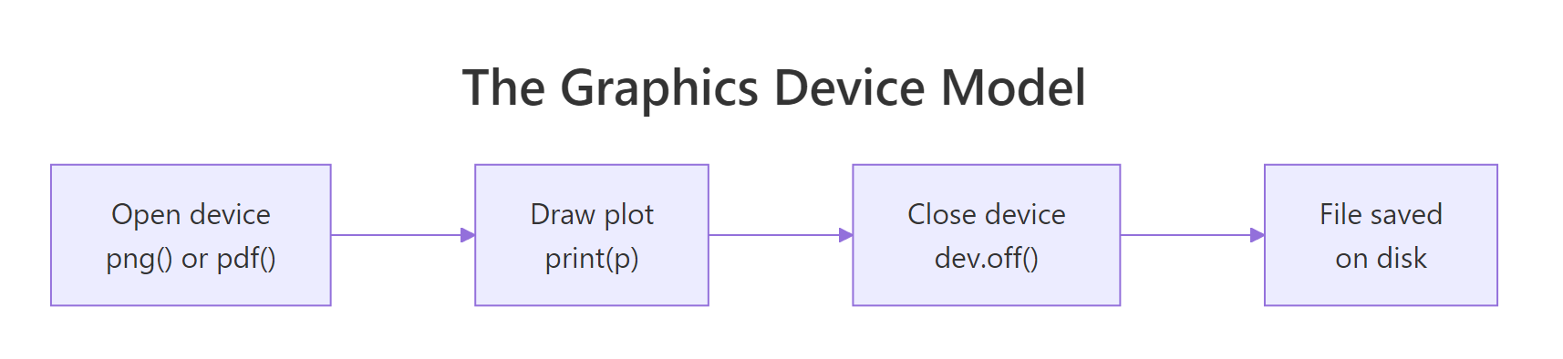
Figure 2: Every save follows the same device cycle: open, draw, close.
Let's do it by hand so the cycle is visible. We open a PNG device with png(), print the plot to send it there, and call dev.off() to close the device. The res argument on png() is that device's version of DPI.
The null device 1 message is R telling you the file device is now closed and drawing has returned to the "null" device, meaning nothing is currently open. That is exactly what you want after a save. Let's confirm the file landed and that no devices are left open.
dev.list() returns NULL, which means there are no open graphics devices, and the file exists on disk. This manual approach is worth knowing for two reasons. First, it works for base R plots too, not just ggplot2 objects, so you can save a hist() or a plot() the same way. Second, it shows you what ggsave() is quietly doing every time you call it.
Try it: Use a pdf() device to save a base R histogram of mtcars$mpg. Remember the three steps: open, draw, close.
Click to reveal solution
Explanation: pdf() opens the device, hist() draws onto it, and dev.off() closes it. Wrapping the close in invisible() just hides the null device message. The device model works for any plot, ggplot2 or base R.
How do you export figures that meet journal specifications?
Academic journals are strict about figures because they have to fit a fixed page layout and print sharply. They almost always specify three things: an exact width (a single column or a double column, quoted in millimetres), a minimum resolution (300 DPI for images, often 600 to 1000 for line art), and an accepted format, most often TIFF or a vector PDF (some journals also take EPS). Meeting these is just a matter of feeding the right numbers to ggsave().
Here are typical widths for a few well-known publishers. Always check the specific journal's author guide, since the numbers vary, but these are close to the common defaults.
| Publisher | Single column | Double column | Minimum resolution |
|---|---|---|---|
| Nature | 89 mm | 183 mm | 300 DPI, 600+ for line art |
| Elsevier | 90 mm | 190 mm | 300 DPI, up to 1000 for line art |
| Science | 55 mm | 121 mm | 300 DPI or higher |
| General rule | about 85 mm | about 170 mm | 300 DPI minimum |
The cleanest way to hit these specs repeatedly is to wrap ggsave() in a small helper that always uses millimetres and a high DPI. Then every figure you export is consistent. Let's write that helper and use it to save a single-column TIFF at 600 DPI.
The helper hides the repetitive arguments so you can think in journal terms ("85 mm single column at 600 DPI") instead of remembering unit flags each time. A single-column figure at 85 mm and 600 DPI comes out to roughly 2000 pixels wide, which comfortably clears most print requirements.
For the sharpest possible text and slightly smaller files, many researchers reach for the ragg package, which provides higher-quality TIFF and PNG devices than base R. Like svglite, it is a local add-on rather than part of the in-browser toolset, so run the block below in your own session.
# Run this in RStudio: ragg renders crisper text and smaller TIFFs
library(ragg)
library(ggplot2)

fig1_ragg <- file.path(tempdir(), "figure-1-ragg.tiff")
agg_tiff(fig1_ragg, width = 85, height = 60, units = "mm",
         res = 600, compression = "lzw")
print(p)
invisible(dev.off())
file.exists(fig1_ragg)
#> [1] TRUE
That uses the device model from the previous section directly: agg_tiff() opens a ragg device, print(p) draws, and dev.off() closes it. If your journal cares about font rendering, or you need to embed specific typefaces, ragg paired with the techniques in Custom Fonts in R Plots gives you the most control. For a fuller treatment of layout, spacing, and polish, see Publication-Ready Figures.
units = "mm" lets you type their number straight into ggsave() with no conversion. Set dpi = 600 for line-heavy plots and you will clear almost any resolution requirement.Try it: Save a double-column figure 170 mm wide at 600 DPI using the save_journal() helper.
Click to reveal solution
Explanation: Passing width_mm = 170 and dpi = 600 to the helper produces a wide, high-resolution TIFF suitable for a two-column journal layout.
Practice Exercises
These combine several ideas from the tutorial. Try each before opening the solution. The exercises use their own variable names so they will not disturb the p object from earlier.
Exercise 1: Export one plot in three formats
Save the plot p as a PNG, a PDF, and a TIFF, all at 6 by 4 inches and 300 DPI. Store the three file paths in my_paths, write them in a loop, then confirm all three files exist with a single check.
Click to reveal solution
Explanation: A single for loop over the paths saves each format, because ggsave() reads the extension every time. all(file.exists(...)) returns one TRUE only if every file was written.
Exercise 2: Hit an exact pixel width
A poster needs a figure exactly 3000 pixels wide at 300 DPI, keeping a 3:2 aspect ratio (so the height is two-thirds of the width). Compute the width in inches from the pixel target, derive the height, then save p to my_poster and confirm it exists.
Click to reveal solution
Explanation: Since pixels equal inches times DPI, the inches you need are the pixel target divided by the DPI, so 3000 / 300 gives 10 inches. The height follows the 3:2 ratio, and ggsave() writes a 3000 by 2000 pixel PNG.
Frequently Asked Questions
Is ggsave() the same as using png() and dev.off()? They produce the same kind of file, but ggsave() is the shortcut. It opens the device, prints your ggplot, and closes the device in one call, and it also guesses the format from the extension. The manual png() then dev.off() route gives you more control and works for base R plots, which ggsave() does not save by default.
Why does my exported plot look blurry or pixelated? Almost always a DPI that is too low. A screenshot or a 72 DPI export has too few pixels for print. Re-save with dpi = 300 (or higher) and set an explicit width and height so the resolution is predictable.
Why does the text in my saved plot look bigger or smaller than on screen? Because ggsave() renders the figure at the exact width and height you asked for, while the on-screen preview stretches the plot to fit your window. Text is sized in fixed points, so the same label takes up a larger share of a small figure and a smaller share of a large one. Decide the width and height you will actually use, then adjust the theme's base_size (for example theme_gray(base_size = 14)) until the text looks right at that size.
What format should I use for a Microsoft Word document? PNG at 300 DPI is the safe, universal choice, since Word handles it everywhere. If you need the figure to stay sharp when someone zooms in, insert a PDF or an EMF instead, because those are vector formats.
How do I control which font appears in the saved file? The base devices can substitute fonts unexpectedly. For reliable fonts, use the ragg devices or the svglite output, then embed or specify the typeface. The Custom Fonts in R Plots tutorial walks through the full setup.
Can I set the size directly in pixels? Yes. Pass units = "px" and give the width and height as pixel counts, for example ggsave("plot.png", width = 1800, height = 1200, units = "px", dpi = 300). The DPI still matters, because it sets how large those pixels are when printed.
Summary
Exporting a plot in R comes down to one call and a handful of choices around it. The figure below maps the moving parts.
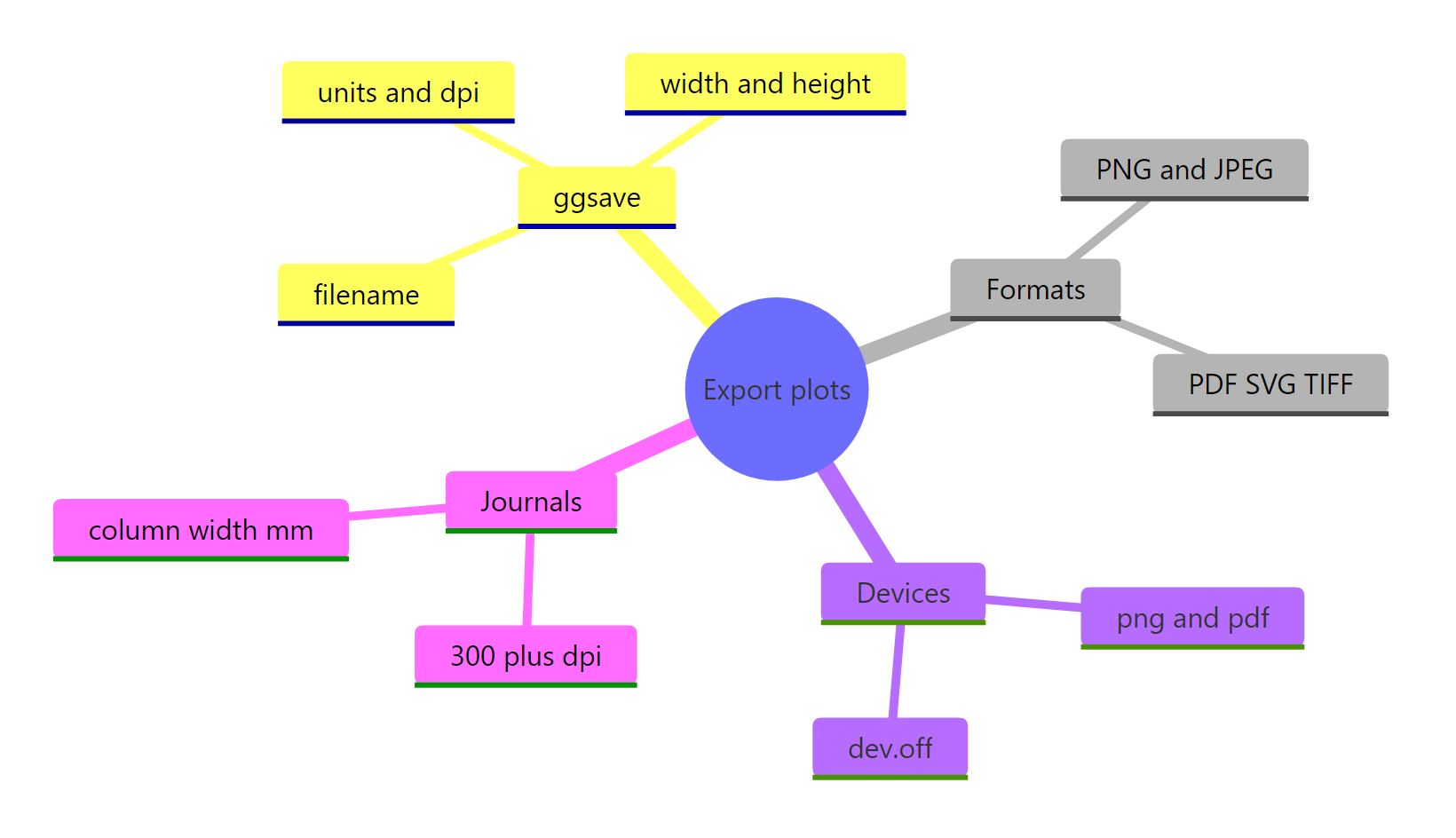
Figure 3: The moving parts of exporting a plot in R.
| Concept | What to remember |
|---|---|
ggsave() |
Saves the last or a named plot; the extension picks the format |
| Width and height | Physical size; set them explicitly, in in, cm, mm, or px |
| DPI | Dots per inch; pixels equal inches times DPI; 300 for print |
| Raster vs vector | PNG/JPEG/TIFF are pixels; PDF/SVG are shapes that never blur |
| Graphics devices | The open, draw, dev.off() cycle that ggsave() wraps |
| Journal specs | Match the column width in mm and use 300 to 600+ DPI TIFF or PDF |
Master ggsave() first, understand DPI so your figures are never blurry, and keep the device model in mind for the cases where you need manual control. With those three, you can produce a file for any target, from a quick Slack preview to a camera-ready journal figure.
References
- ggplot2 documentation. ggsave(): Save a ggplot with sensible defaults. Link
- R Core Team. grDevices: The PNG and other bitmap devices. Link
- Wickham, H., Navarro, D., and Pedersen, T. L. ggplot2: Elegant Graphics for Data Analysis. Link
- ragg package documentation. Graphic devices based on AGG. Link
- svglite package documentation. An SVG graphics device. Link
- Wickham, H., and Grolemund, G. R for Data Science: Communication. Link
- PLOS ONE. Figure preparation guidelines. Link
Continue Learning
- ggsave() in R: Save Plots to PNG, PDF, and SVG - a focused deep dive on every
ggsave()argument. - Publication-Ready Figures in R - polish, layout, and styling for figures headed to print.
- Custom Fonts in R Plots - get the exact typeface you want into your exported files.