Custom Fonts in R Plots: systemfonts, ragg and showtext
Getting a specific typeface into an R plot means going past R's three built-in font families. Three modern packages fix that: systemfonts finds the fonts already on your machine and ragg renders them at high quality, while showtext pulls in any Google Font you lack.
Why won't R just use the font I want?
You set family = "Lato" in your plot, run it, and the text comes out looking exactly the same as before. This is the classic first surprise with fonts in R, and it is not your fault. The font on a plot is chosen by the graphics device, the thing that actually turns your plot into pixels or PDF, not by ggplot2 itself. For years the default devices had awkward font handling, so a name they did not recognise was quietly swapped for a default.
Before we fix that, let's see what R gives you for free. Every R graphics device understands exactly three portable family names. Run this to see them.
Those three names are aliases. "sans" means "the device's default sans-serif" (usually something Arial-like), "serif" means a Times-like serif, and "mono" a fixed-width font. They always work because the device maps them to whatever it has. Anything else, a real named font like Georgia or Lato, needs the tools in this tutorial.
Let's prove the three aliases do something. We build one scatterplot and switch its whole font to serif with base_family, the argument every built-in theme accepts.
The plot below renders the same data three times so you can compare the aliases directly. The sans panel is clean and modern, the serif panel has small strokes at the ends of letters, and the mono panel gives every character the same width.
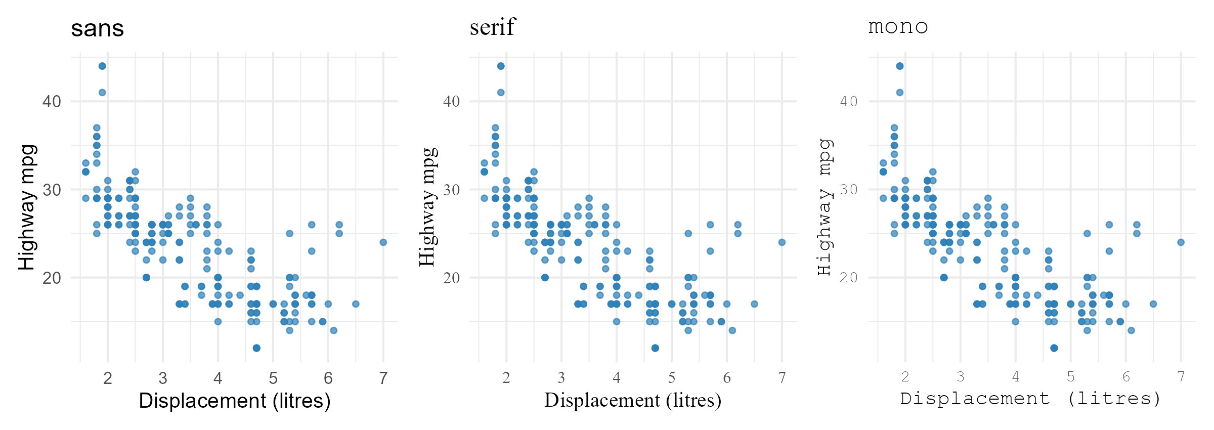
Figure 1: R's three portable font families, applied to the same plot with base_family.
family = "Georgia", something has to find a Georgia file on disk and hand its glyphs to the device. That lookup step is exactly what systemfonts, ragg and showtext handle for you.Try it: Render p with the "mono" family instead of serif and see the fixed-width axis numbers.
Click to reveal solution
Explanation: base_family sets one font for every text element in the theme at once, so a single word changes the entire plot.
How do I control fonts inside ggplot with element_text()?
base_family is the blunt instrument: one font for everything. Most of the time you want finer control, a serif title over mono axis labels, for example. In ggplot2 that control lives in one function: element_text(). Any text element in a theme, the title, the axis labels, the legend, is styled by handing it an element_text().
The function takes a handful of arguments. The two you will use most are family (the typeface) and face (plain, bold, italic, or bold.italic). Here we give the title a bold serif and both axes a grey mono.
Each line targets one element by name and describes how its text should look. plot.title gets the serif treatment, while axis.title (the axis names) and axis.text (the numbers) share the mono look. The result is a plot with a deliberate typographic hierarchy.
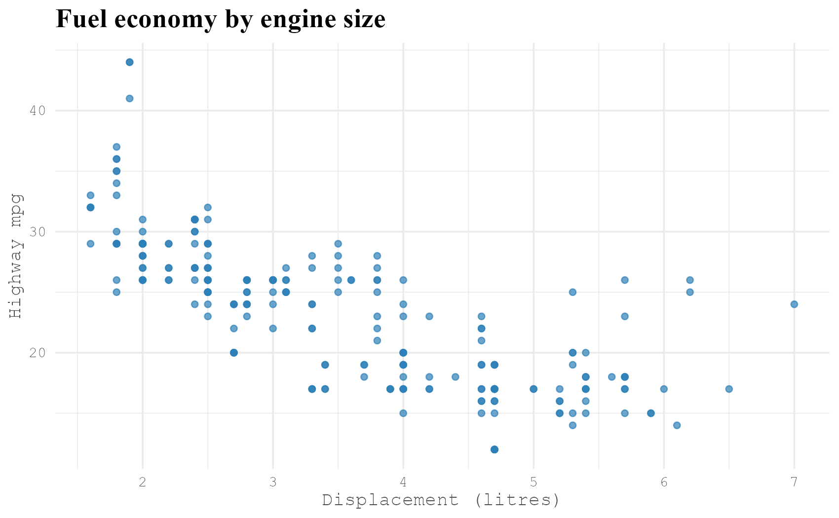
Figure 2: element_text() styles each text element independently.
Setting a family on every element by hand gets repetitive. Theme elements inherit, so you can set a default once on the root text element and then override only what differs. Here every text starts as serif, and just the title adds bold.
There is one place element_text() does not reach: text you draw inside the panel with geom_text() or geom_label(). Those are geoms, not theme elements, so they carry their own family and fontface arguments. Notice we use fontface here, not face, a small naming quirk worth remembering.
We first build label_df, the average position of each vehicle class, then drop a bold mono label at each of those points. The family and fontface arguments belong to geom_text() directly, which is why theme settings never touch them.
Here are the arguments you will reach for inside element_text().
| Argument | Controls | Example values |
|---|---|---|
| family | the typeface | "serif", "mono", "Georgia" |
| face | weight and slant | "plain", "bold", "italic", "bold.italic" |
| size | point size | 14 |
| color | text colour | "grey30" |
| angle | rotation in degrees | 45 |
| hjust | horizontal alignment | 0, 0.5, 1 |
Try it: Change the geom_text() labels to a serif italic style.
Click to reveal solution
Explanation: geom_text() takes family and fontface on the geom itself, so in-panel text is styled separately from the theme.
What fonts does my computer already have? (systemfonts)
So far every font has been one of the three portable aliases. To use a real named font you need to know two things: which fonts your machine actually has, and where their files live. The systemfonts package answers both. It scans your operating system's font folders and is the engine the modern R graphics stack uses to turn a family name into a file.
install.packages(c("systemfonts", "ragg", "showtext")).Start by listing what you have. system_fonts() returns one row per font file, with columns describing each one.
library(systemfonts)

fonts <- system_fonts()
# Which columns describe each font?
colnames(fonts)
#>  [1] "path"      "index"     "name"      "family"    "style"     "weight"    "width"     "italic"
#>  [9] "monospace" "variable"
The two columns you care about most are family (the name you type into a plot) and path (the file on disk). Filter to a family you have to see its available styles. On Windows, Georgia ships with the system, so it makes a good example.
fonts |>
  filter(family == "Georgia") |>
  select(family, style, weight, italic)
#> # A tibble: 4 × 4
#>   family  style       weight italic
#>   <chr>   <chr>       <ord>  <lgl>
#> 1 Georgia Regular     normal FALSE
#> 2 Georgia Bold        bold   FALSE
#> 3 Georgia Bold Italic bold   TRUE
#> 4 Georgia Italic      normal TRUE
Georgia comes in four styles, and each is a separate file. That matters, because "bold" is not a switch you flip, it is a different font file that systemfonts has to locate. You can see it do exactly that with match_fonts(), which resolves a family name plus a weight to the file that will actually be used.
match_fonts("Georgia", weight = "bold")$path
#> [1] "C:\\Windows\\Fonts\\georgiab.ttf"
That path, georgiab.ttf, is the bold Georgia file. This is the whole game: a name in, a file out. Figure 3 shows the pipeline end to end.

Figure 3: How a family name becomes rendered text.
Sometimes you want a name for a weight that has no standard alias, a light or semibold cut. register_variant() lets you create your own family name that points at a specific weight, so you can then use it like any other font.
register_variant("Segoe Light", family = "Segoe UI", weight = "light")

"Segoe Light" %in% registry_fonts()$family
#> [1] TRUE
Now family = "Segoe Light" will render Segoe UI at its light weight anywhere you use it.
Try it: From system_fonts(), keep only the monospace fonts and look at their family names.
# Your turn: filter fonts to rows where monospace is TRUE,
# then look at the unique family names. Which mono fonts do you have?
Click to reveal solution
fonts |>
  filter(monospace) |>
  distinct(family) |>
  head(5)
#> # A tibble: 5 × 1
#>   family
#>   <chr>
#> 1 Consolas
#> 2 Courier New
#> 3 Lucida Console
#> 4 MS Gothic
#> 5 NSimSun
Explanation: system_fonts() flags fixed-width fonts in a monospace column, so filtering on it lists exactly the mono families you can use. Your list will depend on what is installed.
How do I render a system font in a saved plot? (ragg)
Knowing you have Georgia is only half the story. The default png() device still may not draw it. This is where ragg comes in. It is a graphics device, a drop-in replacement for png(), built on the AGG rendering library. Crucially, ragg asks systemfonts to resolve every family name, so any font on your machine works with no extra setup. You write base_family = "Georgia" and Georgia appears.
You use ragg the way you use png(): open the device, print your plot, close the device. The agg_png() function even accepts a res argument so text scales correctly at high resolution.
library(ragg)

p_geo <- ggplot(mpg, aes(displ, hwy)) +
  geom_point(color = "#2c7fb8", alpha = 0.7) +
  labs(title = "Engine size vs highway mpg (Georgia)",
       x = "Displacement (litres)", y = "Highway mpg") +
  theme_minimal(base_size = 14, base_family = "Georgia")

agg_png("georgia_plot.png", width = 1600, height = 1000, res = 200)
print(p_geo)
invisible(dev.off())

file.exists("georgia_plot.png")
#> [1] TRUE
Open georgia_plot.png and you will see the real Georgia typeface, with its distinctive numerals that dip below the baseline. That is a font ragg found through systemfonts, rendered faithfully.
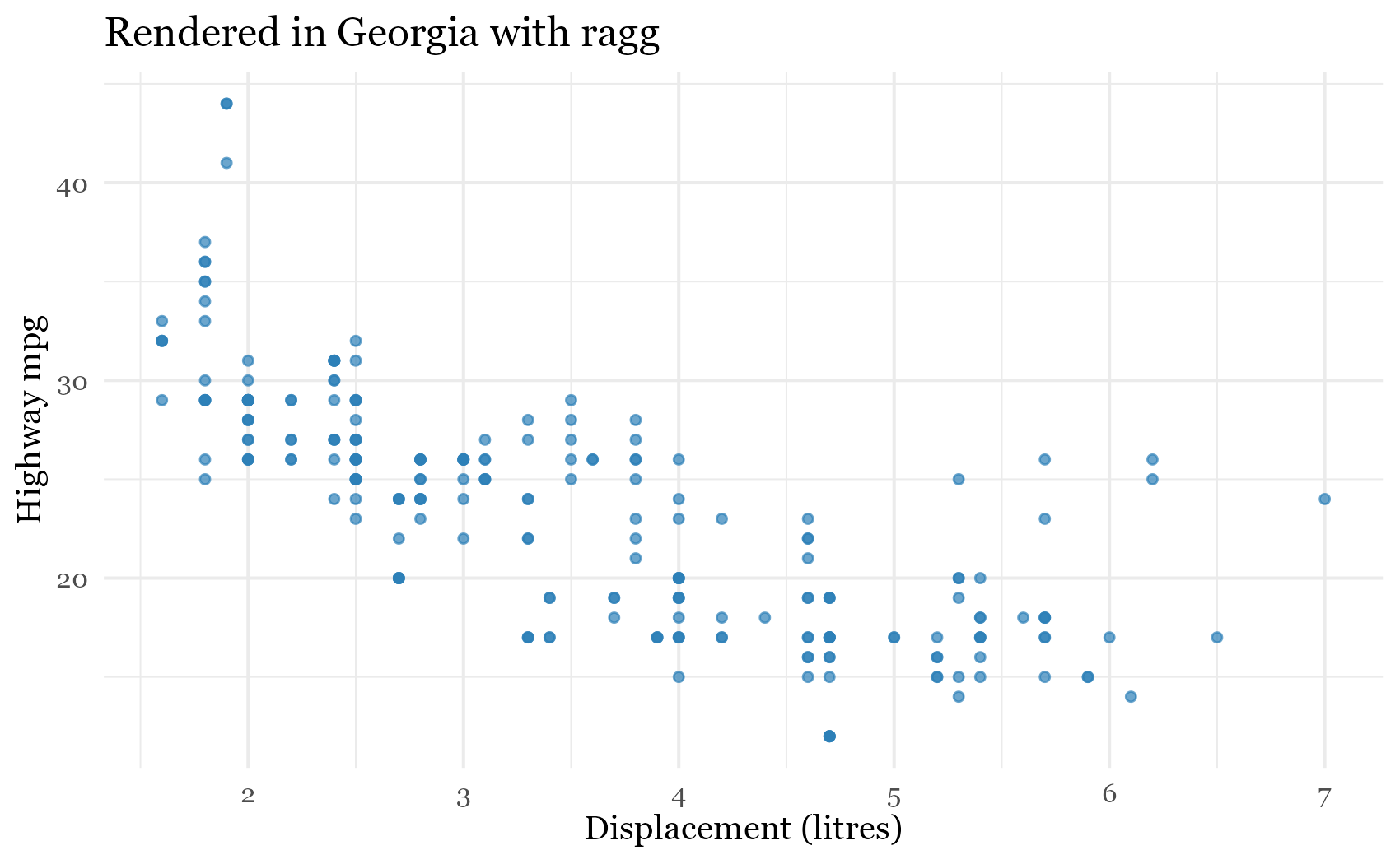
Figure 4: A system font, Georgia, rendered by ragg with no extra configuration.
You rarely want to type agg_png() around every plot. Two settings make ragg your default. In a report, tell knitr to use it for every chunk. In RStudio, switch the graphics backend once.
knitr::opts_chunk$set(dev = "ragg_png")Try it: Render the same plot in Verdana, another font that ships with Windows.
# Your turn: change base_family to "Verdana" and re-render.
# Tip: first confirm you actually have the font.
Click to reveal solution
# swap the base_family, everything else stays the same
p_verd <- p_geo + theme_minimal(base_size = 14, base_family = "Verdana")
"Verdana" %in% system_fonts()$family   # confirm you actually have it
#> [1] TRUE
Explanation: Because ragg resolves names through systemfonts, changing base_family to any installed family is all it takes. Checking membership first avoids a silent fallback when the font is missing.
How do I use a Google Font without installing it? (showtext)
ragg is the right answer when the font lives on your machine. But what about a font you have seen online and not installed, like most of the Google Fonts library? Installing a font system-wide just to try it is a hassle, and it does not help a teammate who lacks the file. The showtext package solves this. It loads a font from a file or straight from Google, then draws text as vector outlines that work on any device.
The workflow has three steps: add the font, turn showtext on, then set its resolution to match the device. That last step is the one everyone forgets.
library(showtext)

font_add_google("Lato", "lato")   # download and register under the name "lato"
showtext_auto()                    # route all plot text through showtext
showtext_opts(dpi = 200)           # match the device resolution (the key step)

p_lato <- ggplot(mpg, aes(displ, hwy)) +
  geom_point(color = "#d95f0e", alpha = 0.7) +
  labs(title = "Engine size vs highway mpg (Lato)",
       x = "Displacement (litres)", y = "Highway mpg") +
  theme_minimal(base_size = 14, base_family = "lato")

agg_png("lato_plot.png", width = 1600, height = 1000, res = 200)
print(p_lato)
invisible(dev.off())

"lato" %in% sysfonts::font_families()
#> [1] TRUE
font_add_google("Lato", "lato") downloads the font and registers it under the short name "lato", which you then pass as base_family. The showtext_opts(dpi = 200) line matches showtext's resolution to the res = 200 on the device, so the text comes out the right size. The result is a clean Lato render with no system install.
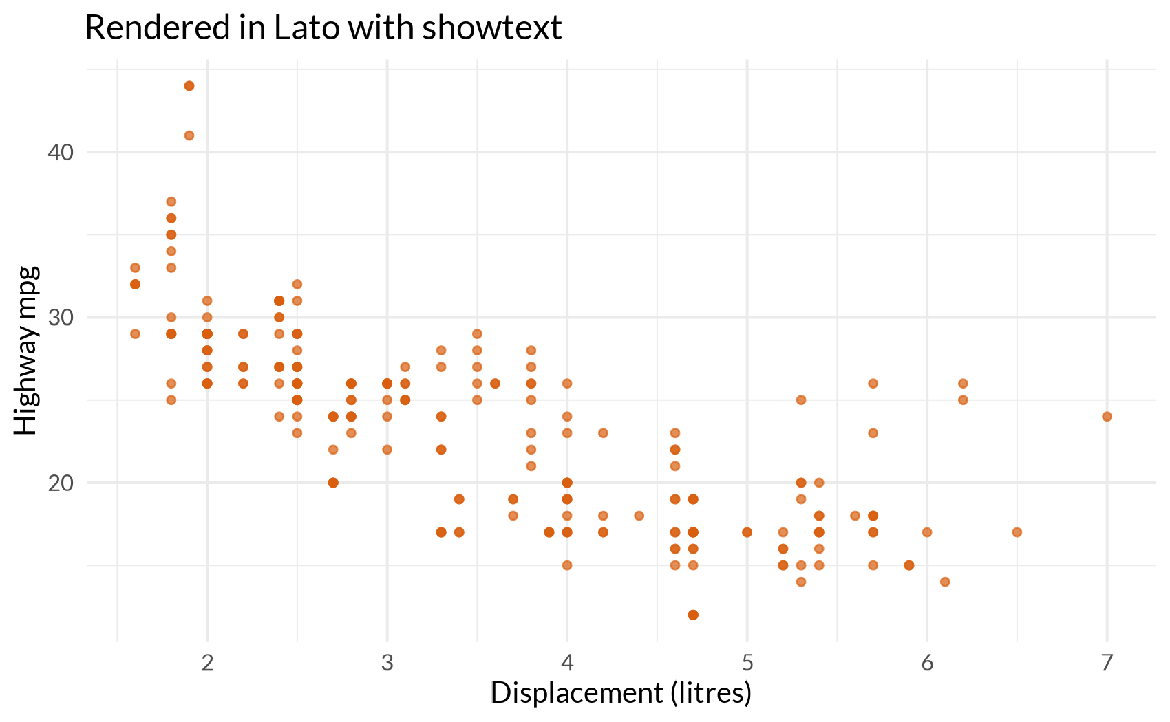
Figure 5: Lato, a Google Font, rendered with showtext and no system install.
showtext is not limited to Google. font_add() loads any font file you point it at, handy for a brand font shipped with your project. When you are done, showtext_auto(FALSE) restores the normal renderer.
sysfonts::font_add("MyGeorgia", regular = "C:/Windows/Fonts/georgia.ttf")
"MyGeorgia" %in% sysfonts::font_families()
#> [1] TRUE

showtext_auto(FALSE) # restore the default renderer when you are doneshowtext_opts(dpi=) does not match your device resolution, text renders far too small or too large. Set the dpi every time and you avoid the most common showtext bug.Try it: Load a different Google Font of your choice and confirm it registered.
# Your turn: pick a font from fonts.google.com (for example "Merriweather"),
# load it with font_add_google(), then check font_families().
Click to reveal solution
font_add_google("Merriweather", "merri")
"merri" %in% sysfonts::font_families()
#> [1] TRUE
Explanation: font_add_google() takes the font's name on Google Fonts and a short alias you choose. After it runs, the alias appears in font_families() and works as a base_family.
ragg or showtext, which should I use?
You now have two ways to get a real font into a plot, and they overlap. The short rule: reach for ragg first, and use showtext for the fonts ragg cannot get. Figure 6 turns that into a decision you can follow in a few seconds.
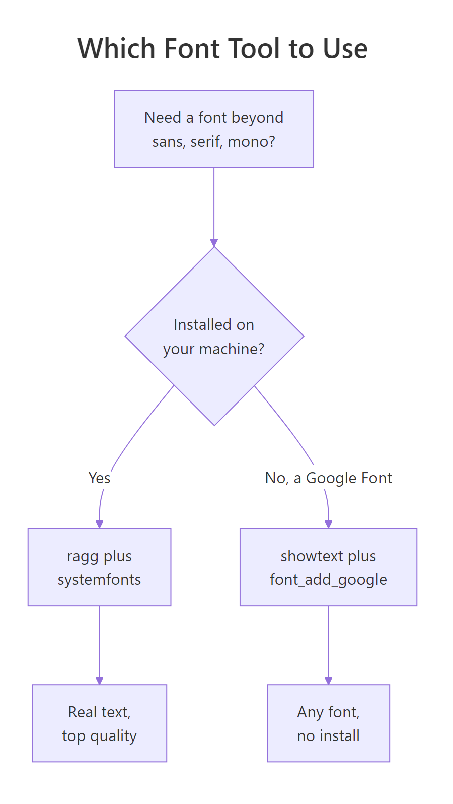
Figure 6: Choosing between ragg and showtext.
The table lays out the trade-offs side by side.
| Question | ragg with systemfonts | showtext |
|---|---|---|
| Which fonts? | any font installed on your machine | any font, Google Fonts included, no install |
| How is text stored? | real, selectable text | vector outlines (shapes) |
| PDF output | keeps real text | text becomes shapes |
| Main gotcha | the font must be installed | set the dpi to match the device |
| Best for | high-quality raster exports, the knitr default | a quick font you have not installed |
For most work, ragg with systemfonts is the better default: it produces real text, top quality, and one setting makes it your global device. showtext earns its place when you want a Google Font or a one-off you would rather not install.
There is also a way to set your font once for a whole session, no matter which device you use. theme_set() changes the default theme every later plot inherits.
Try it: Set every plot in your session to a mono font, then reset to the ggplot2 default.
Click to reveal solution
Explanation: theme_set() replaces the active default theme, so the font applies to every later plot until you set it back.
Practice Exercises
These combine the ideas above. Each solution uses only functions from this tutorial. Use fresh variable names so you do not overwrite the plots from earlier.
Exercise 1: Build a typographic hierarchy
Style a scatterplot of displ against hwy so the title is a bold serif and both axis titles and axis text are mono grey. Use only element_text() in a theme() call.
Click to reveal solution
Explanation: Each element_text() targets one element, so the title and the axes can carry different fonts in the same plot.
Exercise 2: Export a bar chart in an installed font at print resolution
Render a bar chart of vehicle class to a PNG in the Trebuchet MS font at 300 dpi using ragg, then confirm the file was written. Save the plot object as p_treb.
Click to reveal solution
p_treb <- ggplot(mpg, aes(class)) +
  geom_bar(fill = "#2c7fb8") +
  labs(title = "Cars per class") +
  theme_minimal(base_size = 14, base_family = "Trebuchet MS")

agg_png("trebuchet_plot.png", width = 1800, height = 1100, res = 300)
print(p_treb)
invisible(dev.off())

file.exists("trebuchet_plot.png")
#> [1] TRUE
Explanation: ragg resolves "Trebuchet MS" through systemfonts and renders it as real text; the res = 300 argument makes the text sharp at print resolution.
Exercise 3: Export a bar chart in a Google Font
Now do the same chart with a Google Font that is not installed. Load Roboto with showtext, set the dpi to match the device, render to PNG, and confirm the family loaded. Save the plot as p_rob.
Click to reveal solution
font_add_google("Roboto", "roboto")
showtext_auto()
showtext_opts(dpi = 200)

p_rob <- ggplot(mpg, aes(class)) +
  geom_bar(fill = "#d95f0e") +
  labs(title = "Cars per class (Roboto)") +
  theme_minimal(base_size = 14, base_family = "roboto")

agg_png("roboto_plot.png", width = 1800, height = 1100, res = 200)
print(p_rob)
invisible(dev.off())

"roboto" %in% sysfonts::font_families()
#> [1] TRUE
showtext_auto(FALSE)
Explanation: showtext downloads Roboto, registers it under the alias "roboto", and draws it as outlines on the ragg canvas, so a font you never installed still appears in the export.
Frequently Asked Questions
Why does my custom font silently fall back to the default? The graphics device could not find a file for the name you gave. Either the font is not installed (check with "Name" %in% systemfonts::system_fonts()$family), or your device does not use systemfonts to resolve names. Switching to ragg fixes the second problem for installed fonts.
Is ragg better than the old cairo or Windows devices? For most raster output, yes. ragg renders through systemfonts so named fonts work without configuration, and its text and anti-aliasing are typically cleaner. It is also the device the tidyverse now recommends as the knitr and RStudio default.
Can I use a Google Font without an internet connection? font_add_google() needs to download the font the first time. Once you have the file, load it offline with font_add("MyFont", regular = "path/to/file.ttf"), or install it on your system and let ragg pick it up.
I set face = "bold" but nothing changed. Why? Bold is a separate font file, not a computed effect. If the family has no bold style on your machine, there is nothing to switch to. Check the available styles with systemfonts::system_fonts() filtered to that family, as in the systemfonts section above.
How do fonts behave when I export to PDF? With ragg you are producing raster images (PNG, TIFF), where the font is baked into pixels. For a PDF, use a device like cairo_pdf() for real embedded text, or accept that showtext turns text into shapes, which always looks right but is not selectable.
Summary
Custom fonts in R come down to three jobs handled by three packages. systemfonts finds and matches the fonts you have and ragg renders them as real text, while showtext fetches the ones you lack.
| Package | Its job | Reach for it when |
|---|---|---|
| systemfonts | finds and matches the fonts on your machine | you want to know what you have, or alias a weight |
| ragg | a fast device that renders those fonts as real text | you want an installed font in a saved plot (the default choice) |
| showtext | loads any font, Google included, and draws it as outlines | you need a font you have not installed |
The mental model to keep: a family name is just a label until something turns it into a file and hands it to the device. Set ragg as your default backend, learn the element_text() arguments for fine control, and keep showtext ready for the day you want a font off Google Fonts.
References
- systemfonts documentation, r-lib. Link. The reference for the functions that find and match fonts:
system_fonts(),match_fonts(), andregister_variant(). - ragg documentation, r-lib. Link. Documents the device functions like
agg_png()and how to make ragg your knitr and RStudio default. - showtext package, Yixuan Qiu. Link. Shows
font_add(),font_add_google(), and the dpi setting with worked examples. - ggplot2 reference, theme elements including element_text(). Link. Lists every argument
element_text()accepts in one place. - Modern Text Features in R, tidyverse blog. Link. The tidyverse team's own walkthrough of systemfonts and ragg, the basis for this workflow.
- Google Fonts library. Link. Browse the library and copy the exact family name you pass to
font_add_google().
Continue Learning
- ggplot2 Colours: how ggplot2 maps colours, the natural companion to font styling.
- R Color Theory for ggplot2: choose palettes that pair well with your typography.
- ggplot2 Cheat Sheet: a quick reference for the themes and geoms used throughout this tutorial.