Chapter 6 Correlation and Simple Linear Regression

6.1 Relationships between two quantitative variables

The independence test in Chapter 5 provided a technique for assessing evidence of a relationship between two categorical variables. The terms relationship and association are synonyms that, in statistics, imply that particular values on one variable tend to occur more often with some other values of the other variable or that knowing something about the level of one variable provides information about the patterns of values on the other variable. These terms are not specific to the “form” of the relationship – any pattern (strong or weak, negative or positive, easily described or complicated) satisfy the definition. There are two other aspects to using these terms in a statistical context. First, they are not directional – an association between \(x\) and \(y\) is the same as saying there is an association between \(y\) and \(x\). Second, they are not causal unless the levels of one of the variables are randomly assigned in an experimental context. We add to this terminology the idea of correlation between variables \(x\) and \(y\). Correlation, in most statistical contexts, is a measure of the specific type of relationship between the variables: the linear relationship between two quantitative variables⁸⁹. So as we start to review these ideas from your previous statistics course, remember that associations and relationships are more general than correlations and it is possible to have no correlation where there is a strong relationship between variables. “Correlation” is used colloquially as a synonym for relationship but we will work to reserve it for its more specialized usage here to refer specifically to the linear relationship.

Assessing and then modeling relationships between quantitative variables drives the rest of the chapters, so we should get started with some motivating examples to start to think about what relationships between quantitative variables “look like”… To motivate these methods, we will start with a study of the effects of beer consumption on blood alcohol levels (BAC, in grams of alcohol per deciliter of blood). A group of \(n=16\) student volunteers at The Ohio State University drank a randomly assigned number of beers⁹⁰. Thirty minutes later, a police officer measured their BAC. Your instincts, especially as well-educated college students with some chemistry knowledge, should inform you about the direction of this relationship – that there is a positive relationship between Beers and BAC. In other words, higher values of one variable are associated with higher values of the other. Similarly, lower values of one are associated with lower values of the other. In fact there are online calculators that tell you how much your BAC increases for each extra beer consumed (for example: http://www.craftbeer.com/beer-studies/blood-alcohol-content-calculator if you plug in 1 beer). The increase in \(y\) (BAC) for a 1 unit increase in \(x\) (here, 1 more beer) is an example of a slope coefficient that is applicable if the relationship between the variables is linear and something that will be fundamental in what is called a simple linear regression model. In a simple linear regression model (simple means that there is only one explanatory variable) the slope is the expected change in the mean response for a one unit increase in the explanatory variable. You could also use the BAC calculator and the models that we are going to develop to pick a total number of beers you will consume and get a predicted BAC, which employs the entire equation we will estimate.

Before we get to the specifics of this model and how we measure correlation, we should graphically explore the relationship between Beers and BAC in a scatterplot. Figure 6.1 shows a scatterplot of the results that display the expected positive relationship. Scatterplots display the response pairs for the two quantitative variables with the explanatory variable on the \(x\)-axis and the response variable on the \(y\)-axis. The relationship between Beers and BAC appears to be relatively linear but there is possibly more variability than one might expect. For example, for students consuming 5 beers, their BACs range from 0.05 to 0.10. If you look at the online BAC calculators, you will see that other factors such as weight, sex, and beer percent alcohol can impact the results. We might also be interested in previous alcohol consumption. In Chapter 8, we will learn how to estimate the relationship between Beers and BAC after correcting or controlling for those “other variables” using multiple linear regression, where we incorporate more than one quantitative explanatory variable into the linear model (somewhat like in the 2-Way ANOVA). Some of this variability might be hard or impossible to explain regardless of the other variables available and is considered unexplained variation and goes into the residual errors in our models, just like in the ANOVA models. To make scatterplots as in Figure 6.1, you can simply⁹¹ use plot(y~x, data=...).

library(readr)
BB <- read_csv("http://www.math.montana.edu/courses/s217/documents/beersbac.csv")

plot(BAC~Beers, data=BB, pch=16, col=30)

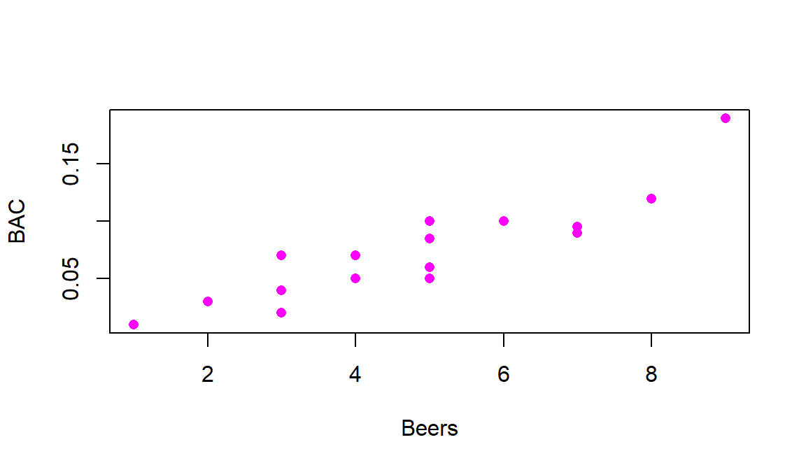
Figure 6.1: Scatterplot of Beers consumed versus BAC.

There are a few general things to look for in scatterplots:

1. Assess the \(\underline{\textbf{direction of the relationship}}\) – is it positive or negative?

2. Consider the \(\underline{\textbf{strength of the relationship}}\). The general idea of assessing strength visually is about how hard or easy it is to see the pattern. If it is hard to see a pattern, then it is weak. If it is easy to see, then it is strong.

3. Consider the \(\underline{\textbf{linearity of the relationship}}\). Does it appear to curve or does it follow a relatively straight line? Curving relationships are called curvilinear or nonlinear and can be strong or weak just like linear relationships – it is all about how tightly the points follow the pattern you identify.

4. Check for \(\underline{\textbf{unusual observations -- outliers}}\) – by looking for points that don’t follow the overall pattern. Being large in \(x\) or \(y\) doesn’t mean that the point is an outlier. Being unusual relative to the overall pattern makes a point an outlier in this setting.

5. Check for \(\underline{\textbf{changing variability}}\) in one variable based on values of the other variable. This will tie into a constant variance assumption later in the regression models.

6. Finally, look for \(\underline{\textbf{distinct groups}}\) in the scatterplot. This might suggest that observations from two populations, say males and females, were combined but the relationship between the two quantitative variables might be different for the two groups.

Going back to Figure 6.1 it appears that there is a moderately strong linear relationship between Beers and BAC – not weak but with some variability around what appears to be a fairly clear to see straight-line relationship. There might even be a hint of a nonlinear relationship in the higher beer values. There are no clear outliers because the observation at 9 beers seems to be following the overall pattern fairly closely. There is little evidence of non-constant variance mainly because of the limited size of the data set – we’ll check this with better plots later. And there are no clearly distinct groups in this plot, possibly because the # of beers was randomly assigned. These data have one more interesting feature to be noted – that subjects managed to consume 8 or 9 beers. This seems to be a large number. I have never been able to trace this data set to the original study so it is hard to know if (1) they had this study approved by a human subjects research review board to make sure it was “safe”, (2) every subject in the study was able to consume their randomly assigned amount, and (3) whether subjects were asked to show up to the study with BACs of 0. We also don’t know the exact alcohol concentration of the beer consumed or volume. So while this is a fun example to start these methods with, a better version of this data set would be nice…

In making scatterplots, there is always a choice of a variable for the \(x\)-axis and the \(y\)-axis. It is our convention to put explanatory or independent variables (the ones used to explain or predict the responses) on the \(x\)-axis. In studies where the subjects are randomly assigned to levels of a variable, this is very clearly an explanatory variable, and we can go as far as making causal inferences with it. In observational studies, it can be less clear which variable explains which. In these cases, make the most reasonable choice based on the observed variables but remember that, when the direction of relationship is unclear, you could have switched the axes and thus the implication of which variable is explanatory.

6.2 Estimating the correlation coefficient

In terms of quantifying relationships between variables, we start with the correlation coefficient, a measure that is the same regardless of your choice of variables as explanatory or response. We measure the strength and direction of linear relationships between two quantitative variables using Pearson’s r or Pearson’s Product Moment Correlation Coefficient. For those who really like acronyms, Wikipedia even suggests calling it the PPMCC. However, its use is so ubiquitous that the lower case r or just “correlation coefficient” are often sufficient to identify that you have used the PPMCC. Some of the extra distinctions arise because there are other ways of measuring correlations in other situations (for example between two categorical variables), but we will not consider them here.

The correlation coefficient, r, is calculated as

\[r=\frac{1}{n-1}\sum^n_{i=1}\left(\frac{x_i-\bar{x}}{s_x}\right) \left(\frac{y_i-\bar{y}}{s_y}\right),\]

where \(s_x\) and \(s_y\) are the standard deviations of \(x\) and \(y\). This formula can also be written as

\[r=\frac{1}{n-1}\sum^n_{i=1}z_{x_i}z_{y_i}\]

where \(z_{x_i}\) is the z-score (observation minus mean divided by standard deviation) for the \(i^{th}\) observation on \(x\) and \(z_{y_i}\) is the z-score for the \(i^{th}\) observation on \(y\). We won’t directly use this formula, but its contents inform the behavior of r. First, because it is a sum divided by (\(n-1\)) it is a bit like an average – it combines information across all observations and, like the mean, is sensitive to outliers. Second, it is a dimension-less measure, meaning that it has no units attached to it. It is based on z-scores which have units of standard deviations of \(x\) or \(y\) so the original units of measurement are cancelled out going into this calculation. This also means that changing the original units of measurement, say from Fahrenheit to Celsius or from miles to km for one or the other variable will have no impact on the correlation. Less obviously, the formula guarantees that r is between -1 and 1. It will attain -1 for a perfect negative linear relationship, 1 for a perfect positive linear relationship, and 0 for no linear relationship. We are being careful here to say linear relationship because you can have a strong nonlinear relationship with a correlation of 0. For example, consider Figure 6.2.

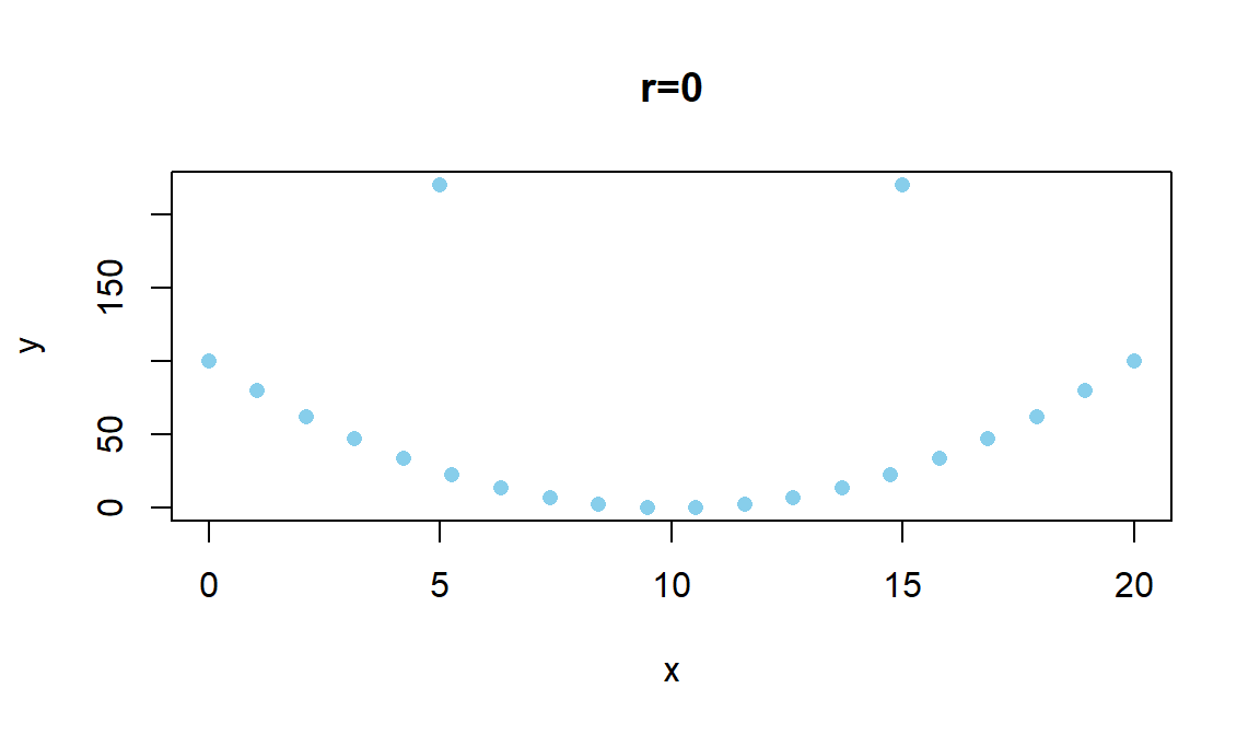
Figure 6.2: Scatterplot of an amusing (and strong) relationship that has \(r=0\).

There are some conditions for trusting the results that the correlation coefficient provides:

1. Two quantitative variables measured.

   • This might seem silly, but categorical variables can be coded numerically and a meaningless correlation can be estimated if you are not careful what you correlate.

2. The relationship between the variables is relatively linear.

   • If the relationship is nonlinear, the correlation is meaningless since it only measures linear relationships and can be misleading if applied to a nonlinear relationship.

3. There should be no outliers.

   • The correlation is very sensitive (technically not resistant) to the impacts of certain types of outliers and you should generally avoid reporting the correlation when they are present.

   • One option in the presence of outliers is to report the correlation with and without outliers to see how they influence the estimated correlation.

The correlation coefficient is dimensionless but larger magnitude values (closer to -1 OR 1) mean stronger linear relationships. A rough interpretation scale based on experiences working with correlations follows, but this varies between fields and types of research and variables measured. It depends on the levels of correlation researchers become used to obtaining, so can even vary within fields. Use this scale until you develop your own experience:

• \(\left|\boldsymbol{r}\right|<0.3\): weak linear relationship,

• \(0.3 < \left|\boldsymbol{r}\right|<0.7\): moderate linear relationship,

• \(0.7 < \left|\boldsymbol{r}\right|<0.9\): strong linear relationship, and

• \(0.9 < \left|\boldsymbol{r}\right|<1.0\): very strong linear relationship.

And again note that this scale only relates to the linear aspect of the relationship between the variables.

When we have linear relationships between two quantitative variables, \(x\) and \(y\), we can obtain estimated correlations from the cor function either using y~x or by running the cor function⁹² on the entire data set. When you run the cor function on a data set it produces a correlation matrix which contains a matrix of correlations where you can triangulate the variables being correlated by the row and column names, noting that the correlation between a variable and itself is 1. A matrix of correlations is useful for comparing more than two variables, discussed below.

library(mosaic)
cor(BAC~Beers, data=BB)

## [1] 0.8943381

cor(BB)

##           Beers       BAC
## Beers 1.0000000 0.8943381
## BAC   0.8943381 1.0000000

Based on either version of using the function, we find that the correlation between Beers and BAC is estimated to be 0.89. This suggests a strong linear relationship between the two variables. Examples are about the only way to build up enough experience to become skillful in using the correlation coefficient. Some additional complications arise in more complicated studies as the next example demonstrates.

Gude et al. (2009) explored the relationship between average summer temperature (degrees F) and area burned (natural log of hectares⁹³ = log(hectares)) by wildfires in Montana from 1985 to 2007. The log-transformation is often used to reduce the impacts of really large observations with non-negative (strictly greater than 0) variables (more on transformations and their impacts on regression models in Chapter 7). Based on your experiences with the wildfire “season” and before analyzing the data, I’m sure you would assume that summer temperature explains the area burned by wildfires. But could it be that more fires are related to having warmer summers? That second direction is unlikely on a state-wide scale but could apply at a particular weather station that is near a fire. There is another option – some other variable is affecting both variables. For example, drier summers might be the real explanatory variable that is related to having both warm summers and lots of fires. These variables are also being measured over time making them examples of time series. In this situation, if there are changes over time, they might be attributed to climate change. So there are really three relationships to explore with the variables measured here (remembering that the full story might require measuring even more!): log-area burned versus temperature, temperature versus year, and log-area burned versus year.

With more than two variables, we can use the cor function on all the variables and end up getting a matrix of correlations or, simply, the correlation matrix. If you triangulate the row and column labels, that cell provides the correlation between that pair of variables. For example, in the first row (Year) and the last column (loghectares), you can find that the correlation coefficient is r=0.362. Note the symmetry in the matrix around the diagonal of 1’s – this further illustrates that correlation between \(x\) and \(y\) does not depend on which variable is viewed as the “response”. The estimated correlation between Temperature and Year is -0.004 and the correlation between loghectares (log-hectares burned) and Temperature is 0.81. So Temperature has almost no linear change over time. And there is a strong linear relationship between loghectares and Temperature. So it appears that temperatures may be related to log-area burned but that the trend over time in both is less clear (at least the linear trends).

mtfires <- read_csv("http://www.math.montana.edu/courses/s217/documents/climateR2.csv")

# natural log transformation of area burned
mtfires$loghectares <- log(mtfires$hectares) 

#Cuts the original hectares data so only log-scale version in tibble
mtfiresR <- mtfires[,-3] 
cor(mtfiresR)

##                   Year Temperature loghectares
## Year         1.0000000  -0.0037991   0.3617789
## Temperature -0.0037991   1.0000000   0.8135947
## loghectares  0.3617789   0.8135947   1.0000000

The correlation matrix alone is misleading – we need to explore scatterplots to check for nonlinear relationships, outliers, and clustering of observations that may be distorting the numerical measure of the linear relationship. The pairs.panels function from the psych package (Revelle 2019) combines the numerical correlation information and scatterplots in one display. There are some options to turn off for the moment but it is an easy function to use to get lots of information in one place. As in the correlation matrix, you triangulate the variables for the pairwise relationship. The upper right panel of Figure 6.3 displays a correlation of 0.36 for Year and loghectares and the lower left panel contains the scatterplot with Year on the \(x\)-axis and loghectares on the \(y\)-axis. The correlation between Year and Temperature is really small, both in magnitude and in display, but appears to be nonlinear (it goes down between 1985 and 1995 and then goes back up), so the correlation coefficient doesn’t mean much here since it just measures the overall linear relationship. We might say that this is a moderate strength (moderately “clear”) curvilinear relationship. In terms of the underlying climate process, it suggests a decrease in summer temperatures between 1985 and 1995 and then an increase in the second half of the data set.

library(psych) 
pairs.panels(mtfiresR, ellipses=F, scale=T, smooth=F, col=0)

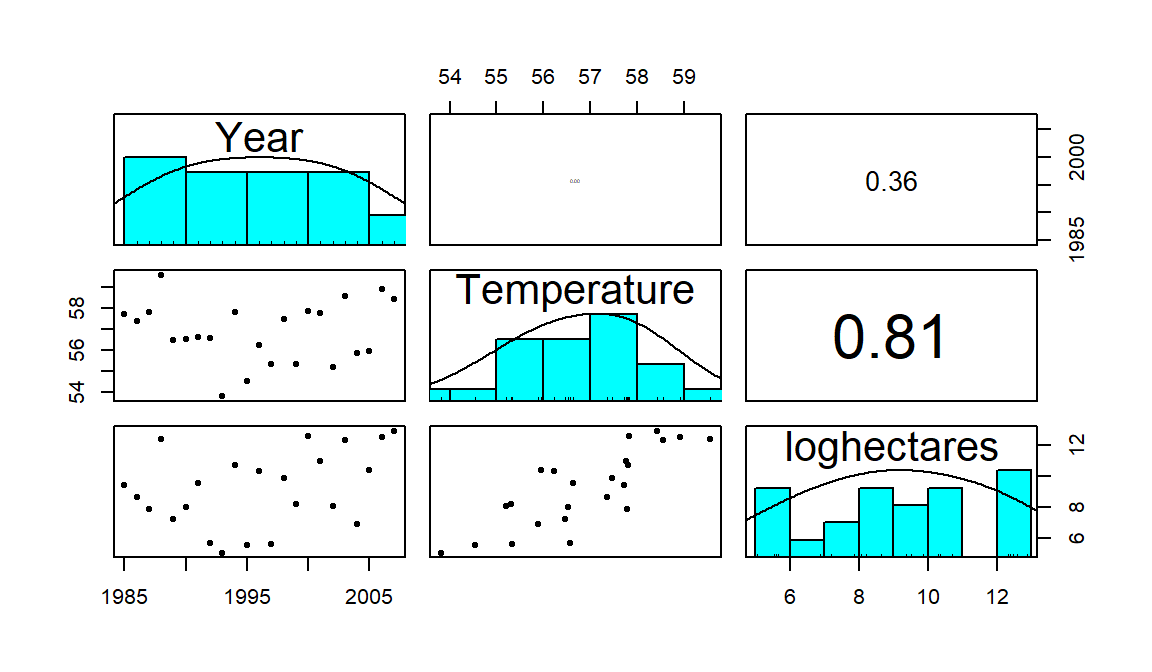
Figure 6.3: Scatterplot matrix of Montana fires data.

As one more example, the Australian Institute of Sport collected data on 102 male and 100 female athletes that are available in the ais data set from the alr3 package (Weisberg (2018), Weisberg (2005)). They measured a variety of variables including the athlete’s Hematocrit (Hc, units of percentage of red blood cells in the blood), Body Fat Percentage (Bfat, units of percentage of total body weight), and height (Ht, units of cm). Eventually we might be interested in predicting Hc based on the other variables, but for now the associations are of interest.

library(alr3)
data(ais)
library(tibble)
ais <- as.tibble(ais)
aisR <- ais[,c("Ht","Hc","Bfat")]
summary(aisR)

##        Ht              Hc             Bfat       
##  Min.   :148.9   Min.   :35.90   Min.   : 5.630  
##  1st Qu.:174.0   1st Qu.:40.60   1st Qu.: 8.545  
##  Median :179.7   Median :43.50   Median :11.650  
##  Mean   :180.1   Mean   :43.09   Mean   :13.507  
##  3rd Qu.:186.2   3rd Qu.:45.58   3rd Qu.:18.080  
##  Max.   :209.4   Max.   :59.70   Max.   :35.520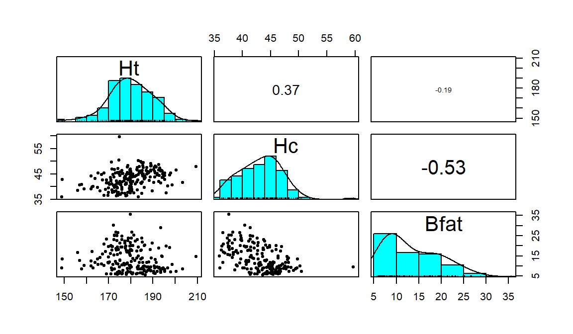

pairs.panels(aisR, scale=T, ellipse=F, smooth=F, col=0)

Figure 6.4: Scatterplot matrix of athlete data.

cor(aisR)

##              Ht         Hc       Bfat
## Ht    1.0000000  0.3711915 -0.1880217
## Hc    0.3711915  1.0000000 -0.5324491
## Bfat -0.1880217 -0.5324491  1.0000000

Ht (Height) and Hc (Hematocrit) have a moderate positive relationship that may contain a slight nonlinearity. It also contains one clear outlier for a middle height athlete (around 175 cm) with an Hc of close to 60% (a result that is extremely high). One might wonder about whether this athlete has been doping or if that measurement involved a recording error. We should consider removing that observation to see how our results might change without it impacting the results. For the relationship between Bfat (body fat) and Hc (hematocrit), that same high Hc value is a clear outlier. There is also a high Bfat (body fat) athlete (35%) with a somewhat low Hc value. This also might be influencing our impressions so we will remove both “unusual” values and remake the plot. The two offending observations were found for individuals numbered 56 and 166 in the data set:

aisR[c(56,166),]

## # A tibble: 2 x 3
##      Ht    Hc  Bfat
##   <dbl> <dbl> <dbl>
## 1  180.  37.6 35.5 
## 2  175.  59.7  9.56

We can create a reduced version of the data (aisR2) by removing those two rows using [-c(56, 166),] and then remake the plot:

aisR2 <- aisR[-c(56,166),] #Removes observations in rows 56 and 166
pairs.panels(aisR2, scale=T, ellipse=F, smooth=F, col=0)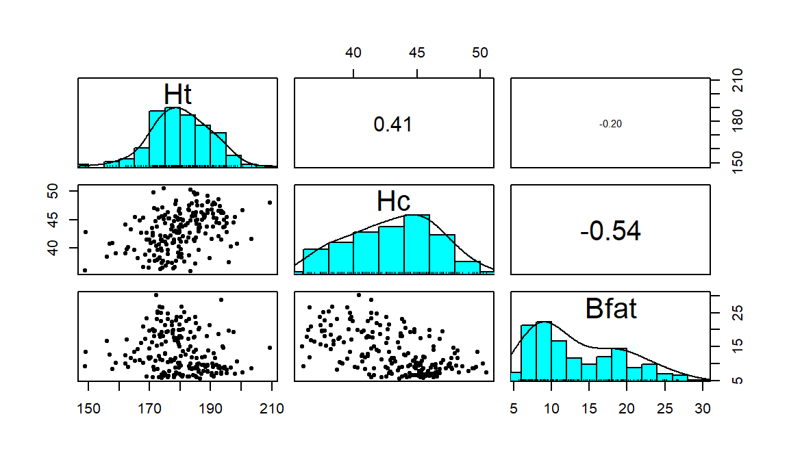

Figure 6.5: Scatterplot matrix of athlete data with two potential outliers removed.

After removing these two unusual observations, the relationships between the variables are more obvious (Figure 6.5). There is a moderate strength, relatively linear relationship between Height and Hematocrit. There is almost no relationship between Height and Body Fat % \((\boldsymbol{r}=-0.20)\). There is a negative, moderate strength, somewhat curvilinear relationship between Hematocrit and Body Fat % \((\boldsymbol{r}=-0.54)\). As hematocrit increases initially, the body fat percentage decreases but at a certain level (around 45% for Hc), the body fat percentage seems to level off. Interestingly, it ended up that removing those two outliers had only minor impacts on the estimated correlations – this will not always be the case.

Sometimes we want to just be able to focus on the correlations, assuming we trust that the correlation is a reasonable description of the results between the variables. To make it easier to see patterns of positive and negative correlations, we can employ a different version of the same display from the corrplot package (Wei and Simko 2017) with the corrplot.mixed function. In this case (Figure 6.6), it tells much the same story but also allows the viewer to easily distinguish both size and direction and read off the numerical correlations if desired.

library(corrplot)
corrplot.mixed(cor(aisR2), upper.col=c("black", "orange"),lower.col=c("black", "orange"))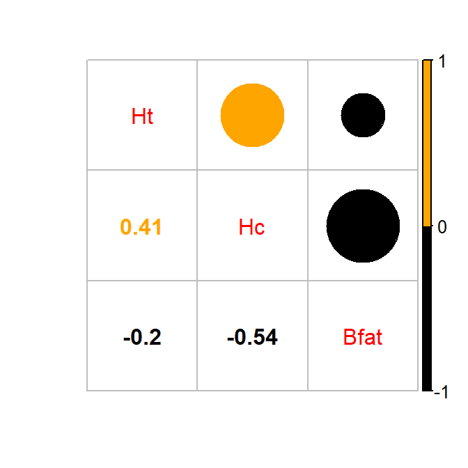

Figure 6.6: Correlation plot of the athlete data with two potential outliers removed. Lighter (orange) circle for positive correlations and black for negative correlations.

6.3 Relationships between variables by groups

In assessing the relationship between variables, incorporating information from a third variable can often enhance the information gathered by either showing that the relationship between the first two variables is the same across levels of the other variable or showing that it differs. When the other variable is categorical (or just can be made categorical), it can be added to scatterplots, changing the symbols and colors for the points based on the different groups. These techniques are especially useful if the categorical variable corresponds to potentially distinct groups in the responses. In the previous example, the data set was built with male and female athletes. For some characteristics, the relationships might be the same for both sexes but for others, there are likely some physiological differences to consider.

We could continue to use the plot function here, but it would require additional lines of code to add these extra features. The scatterplot function from the car package (Fox, Weisberg, and Price (2018), Fox and Weisberg (2011)) makes it easy to incorporate information from an additional categorical variable. We’ll add to our regular formula idea (y~x) the vertical line “|” followed by the categorical variable z, such as y~x|z. As noted earlier, in statistics, “|” means “to condition on” or, here, consider the relationship between \(y\) and \(x\) by groups in \(z\). The other options are mainly to make it easier to read the information in the plot… Using this enhanced notation, Figure 6.7 displays the Height and Hematocrit relationship with information on the sex of the athletes where sex was coded 0 for males and 1 for females.

Figure 6.7: Scatterplot of athlete’s height and hematocrit by sex of athletes. Males were coded as 0s and females as 1s.

aisR2 <- ais[-c(56,166),c("Ht","Hc","Bfat","Sex")]
library(car)
aisR2$Sex <- factor(aisR2$Sex)
scatterplot(Hc~Ht|Sex, data=aisR2, pch=c(3,21), regLine=F, smooth=F,
            boxplots="xy", main="Scatterplot of Height vs Hematocrit by Sex") 
# pch=c(3,21) provides two different symbols that are easy to distinguish. 
# Drop this option or add more numbers to the list if you have more than 2 groups.

Adding the grouping information really changes the impressions of the relationship between Height and Hematocrit – within each sex, there is little relationship between the two variables. The overall relationship is of moderate strength and positive but the subgroup relationships are weak at best. The overall relationship is created by inappropriately combining two groups that had different means in both the \(x\) and \(y\) directions. Men have higher mean heights and hematocrit values than women and putting them together in one large group creates the misleading overall relationship⁹⁴.

To get the correlation coefficients by groups, we can subset the data set using a logical inquiry on the Sex variable in the updated aisR2 data set, using Sex==0 in the subset function to get a tibble with male subjects only and Sex==1 for the female subjects, then running the cor function on each version of the data set:

cor(Hc~Ht, data=subset(aisR2,Sex==0)) #Males only

## [1] -0.04756589

cor(Hc~Ht, data=subset(aisR2,Sex==1)) #Females only

## [1] 0.02795272

These results show that \(\boldsymbol{r}=-0.05\) for Height and Hematocrit for males and \(\boldsymbol{r}=0.03\) for females. The first suggests a very weak negative linear relationship and the second suggests a very weak positive linear relationship. The correlation when the two groups were combined (and group information was ignored!) was that \(\boldsymbol{r}=0.37\). So one conclusion here is that correlations on data sets that contain groups can be very misleading (if the groups are ignored). It also emphasizes the importance of exploring for potential subgroups in the data set – these two groups were not obvious in the initial plot, but with added information the real story became clear.

For the Body Fat vs Hematocrit results in Figure 6.8, with an overall correlation of \(\boldsymbol{r}=-0.54\), the subgroup correlations show weaker relationships that also appear to be in different directions (\(\boldsymbol{r}=0.13\) for men and \(\boldsymbol{r}=-0.17\) for women). This doubly reinforces the dangers of aggregating different groups and ignoring the group information.

cor(Hc~Bfat, data=subset(aisR2,Sex==0)) #Males only

## [1] 0.1269418

cor(Hc~Bfat, data=subset(aisR2,Sex==1)) #Females only

## [1] -0.1679751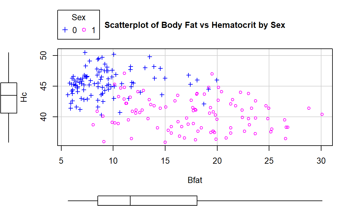

Figure 6.8: Scatterplot of athlete’s body fat and hematocrit by sex of athletes. Males were coded as 0s and females as 1s.

scatterplot(Hc~Bfat|Sex, data=aisR2, pch=c(3,21), regLine=F, smooth=F,
            boxplots="xy", main="Scatterplot of Body Fat vs Hematocrit by Sex")

One final exploration for these data involves the body fat and height relationship displayed in Figure 6.9. This relationship shows an even greater disparity between overall and subgroup results. The overall relationship is characterized as a weak negative relationship \((\boldsymbol{r}=-0.20)\) that is not clearly linear or nonlinear. The subgroup relationships are both clearly positive with a stronger relationship for men that might also be nonlinear (for the linear relationships \(\boldsymbol{r}=0.45\) for women and \(\boldsymbol{r}=0.20\) for men). Especially for female athletes, those that are taller seem to have higher body fat percentages. This might be related to the types of sports they compete in – that would be another categorical variable we could incorporate… Both groups also seem to demonstrate slightly more variability in Body Fat associated with taller athletes (each sort of “fans out”).

cor(Bfat~Ht, data=subset(aisR2,Sex==0)) #Males only

## [1] 0.1954609

cor(Bfat~Ht, data=subset(aisR2,Sex==1)) #Females only

## [1] 0.4476962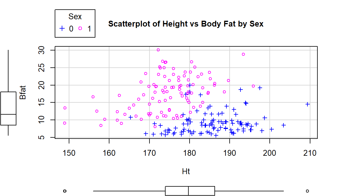

Figure 6.9: Scatterplot of athlete’s body fat and height by sex.

scatterplot(Bfat~Ht|Sex, data=aisR2, pch=c(3,21), regLine=F, smooth=F,
            boxplots="xy", main="Scatterplot of Height vs Body Fat by Sex")

In each of these situations, the sex of the athletes has the potential to cause misleading conclusions if ignored. There are two ways that this could occur – if we did not measure it then we would have no hope to account for it OR we could have measured it but not adjusted for it in our results, as was done initially. We distinguish between these two situations by defining the impacts of this additional variable as either a confounding or lurking variable:

• Confounding variable: affects the response variable and is related to the explanatory variable. The impacts of a confounding variable on the response variable cannot be separated from the impacts of the explanatory variable.

• Lurking variable: a potential confounding variable that is not measured and is not considered in the interpretation of the study.

Lurking variables show up in studies sometimes due to lack of knowledge of the system being studied or a lack of resources to measure these variables. Note that there may be no satisfying resolution to the confounding variable problem but that it is better to have measured it and know about it than to have it remain a lurking variable.

To help think about confounding and lurking variables, consider the following situation. On many highways, such as Highway 93 in Montana and north into Canada, recent construction efforts have been involved in creating safe passages for animals by adding fencing and animal crossing structures. These structures both can improve driver safety, save money from costs associated with animal-vehicle collisions, and increase connectivity of animal populations. Researchers (such as Clevenger and Waltho (2005)) involved in these projects are interested in which characteristics of underpasses lead to the most successful structures, mainly measured by rates of animal usage (number of times they cross under the road). Crossing structures are typically made using culverts and those tend to be cylindrical. Researchers are interested in studying the effect of height and width of crossing structures on animal usage. Unfortunately, all the tallest structures are also the widest structures. If animals prefer the tall and wide structures, then there is no way to know if it is due to the height or width of the structure since they are confounded. If the researchers had only measured width, then they might assume that it is the important characteristic of the structures but height could be a lurking variable that really was the factor related to animal usage of the structures. This is an example where it may not be possible to design a study that prevents confounding of the two variables height and width. If the researchers could control the height and width of the structures independently, then they could randomly assign both variables to make sure that some narrow structures are installed that are tall and some that are short. Additionally, they would also want to have some wide structures that are short and some are tall. Careful design of studies can prevent confounding of variables if they are known in advance and it is possible to control them, but in observational studies the observed combinations of variables are uncontrollable. This is why we need to employ additional caution in interpreting results from observational studies. Here that would mean that even if width was found to be a predictor of animal usage, we would likely want to avoid saying that width of the structures caused differences in animal usage.

6.4 Inference for the correlation coefficient

We used bootstrapping briefly in Chapter 2 to generate nonparametric confidence intervals based on the middle 95% of the bootstrapped version of the statistic. Remember that bootstrapping involves sampling with replacement from the data set and creates a distribution centered near the statistic from the real data set. This also mimics sampling under the alternative as opposed to sampling under the null as in our permutation approaches. Bootstrapping is particularly useful for making confidence intervals where the distribution of the statistic may not follow a named distribution. This is the case for the correlation coefficient which we will see shortly.

The correlation is an interesting summary but it is also an estimator of a population parameter called \(\rho\) (the symbol rho), which is the population correlation coefficient. When \(\rho = 1\), we have a perfect positive linear relationship in the population; when \(\rho=-1\), there is a perfect negative linear relationship in the population; and when \(\rho=0\), there is no linear relationship in the population. Therefore, to test if there is a linear relationship between two quantitative variables, we use the null hypothesis \(H_0: \rho=0\) (tests if the true correlation, \(\rho\), is 0 – no linear relationship). The alternative hypothesis is that there is some (positive or negative) relationship between the variables in the population, \(H_A: \rho \ne 0\). The distribution of the Pearson correlation coefficient can be complicated in some situations, so we will use bootstrapping methods to generate confidence intervals for \(\rho\) based on repeated random samples with replacement from the original data set. If the \(C\%\) confidence interval contains 0, then we would find little to no evidence against the null hypothesis since 0 is in the interval of our likely values for \(\rho\). If the \(C\%\) confidence interval does not contain 0, then we would find strong evidence against the null hypothesis. Along with its use in testing, it is also interesting to be able to generate a confidence interval for \(\rho\) to provide an interval where we are \(C\%\) confident that the true parameter lies.

The beers and BAC example seemed to provide a strong relationship with \(\boldsymbol{r}=0.89\). As correlations approach -1 or 1, the sampling distribution becomes more and more skewed. This certainly shows up in the bootstrap distribution that the following code produces (Figure 6.10). Remember that bootstrapping utilizes the resample function applied to the data set to create new realizations of the data set by re-sampling with replacement from those observations. The bold vertical line in Figure 6.10 corresponds to the estimated correlation \(\boldsymbol{r}=0.89\) and the distribution contains a noticeable left skew with a few much smaller \(T^*\text{'s}\) possible in bootstrap samples. The \(C\%\) confidence interval is found based on the middle \(C\%\) of the distribution or by finding the values that put \((100-C)/2\) into each tail of the distribution with the qdata function.

Tobs <- cor(BAC~Beers, data=BB); Tobs

## [1] 0.8943381

set.seed(614)
B <- 1000
Tstar <- matrix(NA, nrow=B)
for (b in (1:B)){
  Tstar[b] <- cor(BAC~Beers, data=resample(BB))
}
quantiles <- qdata(Tstar, c(0.025,0.975)) #95% Confidence Interval

quantiles

##        quantile     p
## 2.5%  0.7633606 0.025
## 97.5% 0.9541518 0.975

par(mfrow=c(1,2))
hist(Tstar, labels=T, ylim=c(0,550))
abline(v=Tobs, col="red", lwd=3)
abline(v=quantiles$quantile, col="blue", lty=2, lwd=3)

plot(density(Tstar), main="Density curve of Tstar")
abline(v=Tobs, col="red", lwd=3)
abline(v=quantiles$quantile, col="blue", lty=2, lwd=3)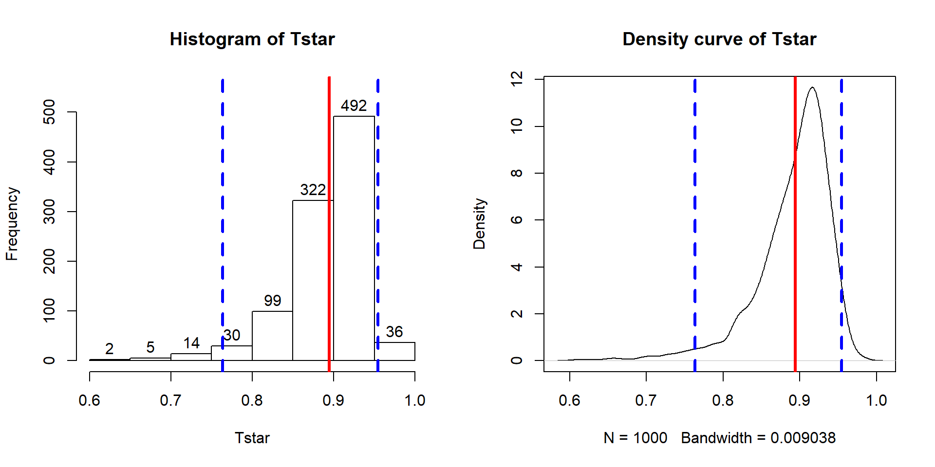

Figure 6.10: Histogram and density curve of the bootstrap distribution of the correlation coefficient with bold vertical line for observed correlation and dashed lines for bounds for the 95% bootstrap confidence interval.

These results tell us that the bootstrap 95% CI is from 0.76 to 0.95 – we are 95% confident that the true correlation between Beers and BAC in all OSU students like those that volunteered for this study is between 0.76 and 0.95. Note that there are no units on the correlation coefficient or in this interpretation of it.

We can also use this confidence interval to test for a linear relationship between these variables.

• \(\boldsymbol{H_0:\rho=0:}\) There is no linear relationship between Beers and BAC in the population.

• \(\boldsymbol{H_A: \rho \ne 0:}\) There is a linear relationship between Beers and BAC in the population.

The 95% confidence level corresponds to a 5% significance level test and if the 95% CI does not contain 0, you know that the p-value would be less than 0.05 and if it does contain 0 that the p-value would be more than 0.05. The 95% CI is from 0.76 to 0.95, which does not contain 0, so we find strong evidence⁹⁵ against the null hypothesis and conclude that there is a linear relationship between Beers and BAC in OSU students. We’ll revisit this example using the upcoming regression tools to explore the potential for more specific conclusions about this relationship. Note that for these inferences to be accurate, we need to be able to trust that the sample correlation is reasonable for characterizing the relationship between these variables along with the assumptions we will discuss below.

In this situation with randomly assigned levels of \(x\) and strong evidence against the null hypothesis of no relationship, we can further conclude that changing beer consumption causes changes in the BAC. This is a much stronger conclusion than we can typically make based on correlation coefficients. Correlations and scatterplots are enticing for infusing causal interpretations in non-causal situations. Statistics teachers often repeat the mantra that correlation is not causation and that generally applies – except when there is randomization involved in the study. It is rarer for researchers either to assign, or even to be able to assign, levels of quantitative variables so correlations should be viewed as non-causal unless the details of the study suggest otherwise.

6.5 Are tree diameters related to tree heights?

In a study at the Upper Flat Creek study area in the University of Idaho Experimental Forest, a random sample of \(n=336\) trees was selected from the forest, with measurements recorded on Douglas Fir, Grand Fir, Western Red Cedar, and Western Larch trees. The data set called ufc is available from the spuRs package (Jones et al. 2018) and contains dbh.cm (tree diameter at 1.37 m from the ground, measured in cm) and height.m (tree height in meters). The relationship displayed in Figure 6.11 is positive, moderately strong with some curvature and increasing variability as the diameter increases. There do not appear to be groups in the data set but since this contains four different types of trees, we would want to revisit this plot by type of tree.

library(spuRs) #install.packages("spuRs")
data(ufc)
ufc <- as_tibble(ufc)
scatterplot(height.m~dbh.cm, data=ufc, smooth=F, regLine=T, pch=16)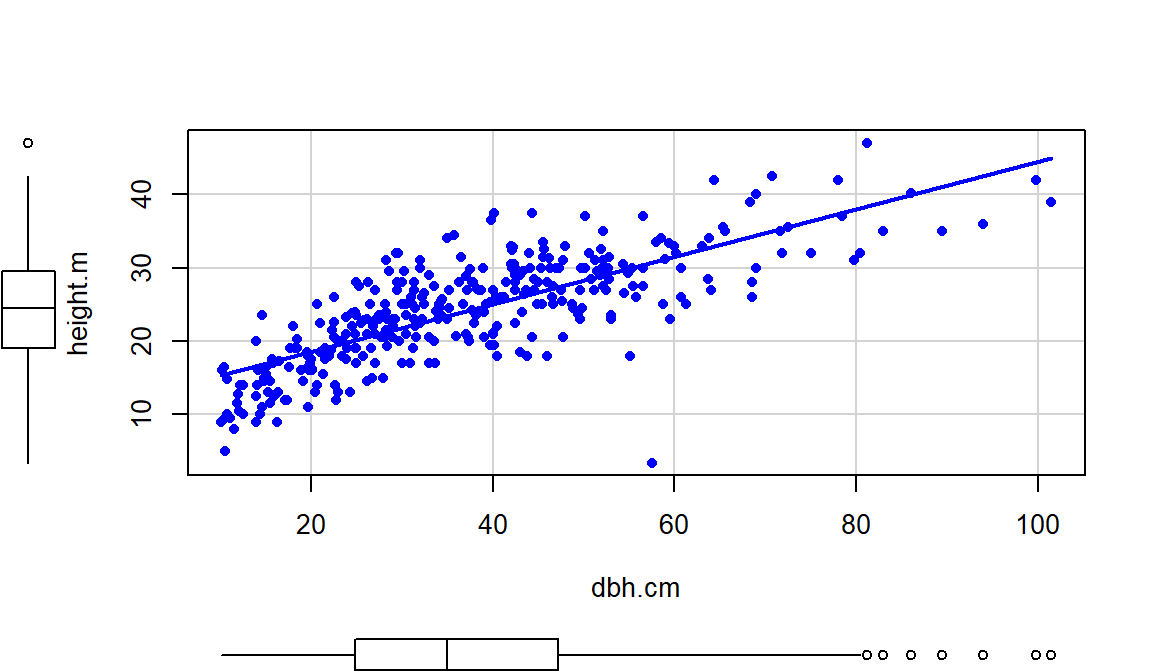

Figure 6.11: Scatterplot of tree heights (m) vs tree diameters (cm).

Of particular interest is an observation with a diameter around 58 cm and a height of less than 5 m. Observing a tree with a diameter around 60 cm is not unusual in the data set, but none of the other trees with this diameter had heights under 15 m. It ends up that the likely outlier is in observation number 168 and because it is so unusual it likely corresponds to either a damaged tree or a recording error.

ufc[168,]

## # A tibble: 1 x 5
##    plot  tree species dbh.cm height.m
##   <int> <int> <fct>    <dbl>    <dbl>
## 1    67     6 WL        57.5      3.4

With the outlier in the data set, the correlation is 0.77 and without it, the correlation increases to 0.79. The removal does not create a big change because the data set is relatively large and the diameter value is close to the mean of the \(x\text{'s}\)⁹⁶ but it has some impact on the strength of the correlation.

cor(dbh.cm~height.m, data=ufc)

## [1] 0.7699552

cor(dbh.cm~height.m, data=ufc[-168,])

## [1] 0.7912053

With the outlier included, the bootstrap 95% confidence interval goes from 0.702 to 0.820 – we are 95% confident that the true correlation between diameter and height in the population of trees is between 0.708 and 0.819. When the outlier is dropped from the data set, the 95% bootstrap CI is 0.753 to 0.826, which shifts the lower endpoint of the interval up, reducing the width of the interval from 0.111 to 0.073. In other words, the uncertainty regarding the value of the population correlation coefficient is reduced. The reason to remove the observation is that it is unusual based on the observed pattern, which implies an error in data collection or sampling from a population other than the one used for the other observations and, if the removal is justified, it helps us refine our inferences for the population parameter. But measuring the linear relationship in these data where there is a clear curve violates one of our assumptions of using these methods – we’ll see some other ways of detecting this issue in Section 6.10 and we’ll try to “fix” this example using transformations in the Chapter 7.

Tobs <- cor(dbh.cm~height.m, data=ufc); Tobs

## [1] 0.7699552

set.seed(208)
par(mfrow=c(2,1))
B <- 1000
Tstar <- matrix(NA, nrow=B)
for (b in (1:B)){
  Tstar[b] <- cor(dbh.cm~height.m, data=resample(ufc))
}
quantiles <- qdata(Tstar, c(.025,.975)) #95% Confidence Interval
quantiles

##        quantile     p
## 2.5%  0.7075771 0.025
## 97.5% 0.8190283 0.975

hist(Tstar, labels=T, xlim=c(0.6,0.9), ylim=c(0,275),
     main="Bootstrap distribution of correlation with all data")
abline(v=Tobs, col="red", lwd=3)
abline(v=quantiles$quantile, col="blue", lty=2, lwd=3)

Tobs <- cor(dbh.cm~height.m, data=ufc[-168,]); Tobs

## [1] 0.7912053

Tstar <- matrix(NA, nrow=B)
for (b in (1:B)){
  Tstar[b] <- cor(dbh.cm~height.m, data=resample(ufc[-168,]))
}
quantiles <- qdata(Tstar, c(.025,.975)) #95% Confidence Interval
quantiles

##        quantile     p
## 2.5%  0.7532338 0.025
## 97.5% 0.8259416 0.975

hist(Tstar, labels=T, xlim=c(0.6,0.9), ylim=c(0,275),
     main= "Bootstrap distribution of correlation without outlier")
abline(v=Tobs, col="red", lwd=3)
abline(v=quantiles$quantile, col="blue", lty=2, lwd=3)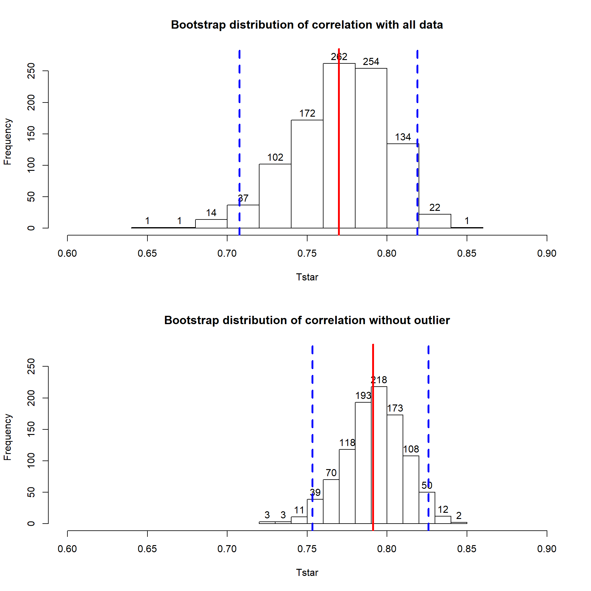

Figure 6.12: Bootstrap distributions of the correlation coefficient for the full data set (top) and without potential outlier included (bottom) with observed correlation (bold line) and bounds for the 95% confidence interval (dashed lines). Notice the change in spread of the bootstrap distributions as well as the different centers.

6.6 Describing relationships with a regression model

When the relationship appears to be relatively linear, it makes sense to estimate and then interpret a line to represent the relationship between the variables. This line is called a regression line and involves finding a line that best fits (explains variation in) the response variable for the given values of the explanatory variable. For regression, it matters which variable you choose for \(x\) and which you choose for \(y\) – for correlation it did not matter. This regression line describes the “effect” of \(x\) on \(y\) and also provides an equation for predicting values of \(y\) for given values of \(x\). The Beers and BAC data provide a nice example to start our exploration of regression models. The beer consumption is a clear explanatory variable, detectable in the story because (1) it was randomly assigned to subjects and (2) basic science supports beer consumption amount being an explanatory variable for BAC. In some situations, this will not be so clear, but look for random assignment or scientific logic to guide your choices of variables as explanatory or response⁹⁷. Regression lines are actually provided by default in the scatterplot function with the reg.line=T option or just omitting reg.line=F from the previous versions of the code since it is a default option to provide the lines.

scatterplot(BAC~Beers, ylim=c(0,.2), xlim=c(0,9), data=BB, pch=16,
            boxplot=F, main="Scatterplot with regression line",
            lwd=2, smooth=F)
abline(v=1:9, col="grey")
abline(h=c(0.05914,0.0771), col="blue", lty=2, lwd=2)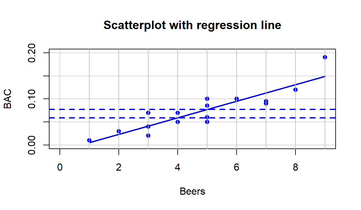

Figure 6.13: Scatterplot with estimated regression line for the Beers and BAC data. Horizontal dashed lines for the predicted BAC for 4 and 5 beers consumed.

The equation for a line is \(y=a+bx\), or maybe \(y=mx+b\). In the version \(mx+b\) you learned that \(m\) is a slope coefficient that relates a change in \(x\) to changes in \(y\) and that \(b\) is a \(y\)-intercept (the value of \(y\) when \(x\) is 0). In Figure 6.13, two extra horizontal lines are added to help you see the defining characteristics of the line. The slope, whatever letter you use, is the change in \(y\) for a one-unit increase in \(x\). Here, the slope is the change in BAC for a 1 beer increase in Beers, such as the change from 4 to 5 beers. The \(y\)-values (blue, dashed lines) for Beers = 4 and 5 go from 0.059 to 0.077. This means that for a 1 beer increase (+1 unit change in \(x\)), the BAC goes up by \(0.077-0.059=0.018\) (+0.018 unit change in \(y\)). We can also try to find the \(y\)-intercept on the graph by looking for the BAC level for 0 Beers consumed. The \(y\)-value (BAC) ends up being around -0.01 if you extend the regression line to Beers=0. You might assume that the BAC should be 0 for Beers=0 but the researchers did not observe any students at 0 Beers, so we don’t really know what the BAC might be at this value. We have to use our line to predict this value. This ends up providing a prediction below 0 – an impossible value for BAC. If the \(y\)-intercept were positive, it would suggest that the students has a BAC over 0 even without drinking.

The numbers reported were very accurate because we weren’t using the plot alone to generate the values – we were using a linear model to estimate the equation to describe the relationship between Beers and BAC. In statistics, we estimate “\(m\)” and “\(b\)”. We also write the equation starting with the \(y\)-intercept and use slightly different notation that allows us to extend to more complicated models with more variables. Specifically, the estimated regression equation is \(\widehat{y} = b_0 + b_1x\), where

• \(\widehat{y}\) is the estimated value of \(y\) for a given \(x\),

• \(b_0\) is the estimated \(y\)-intercept (predicted value of \(y\) when \(x\) is 0),

• \(b_1\) is the estimated slope coefficient, and

• \(x\) is the explanatory variable.

One of the differences between when you learned equations in algebra classes and our situation is that the line is not a perfect description of the relationship between \(x\) and \(y\) – it is an “on average” description and will usually leave differences between the line and the observations, which we call residuals \((e = y-\widehat{y})\). We worked with residuals in the ANOVA⁹⁸ material. The residuals describe the vertical distance in the scatterplot between our model (regression line) and the actual observed data point. The lack of a perfect fit of the line to the observations distinguishes statistical equations from those you learned in math classes. The equations work the same, but we have to modify interpretations of the coefficients to reflect this.

We also tie this estimated model to a theoretical or population regression model:

\[y_i = \beta_0 + \beta_1x_i+\varepsilon_i\]

where:

• \(y_i\) is the observed response for the \(i^{th}\) observation,

• \(x_i\) is the observed value of the explanatory variable for the \(i^{th}\) observation,

• \(\beta_0 + \beta_1x_i\) is the true mean function evaluated at \(x_i\),

• \(\beta_0\) is the true (or population) \(y\)-intercept,

• \(\beta_1\) is the true (or population) slope coefficient, and

• the deviations, \(\varepsilon_i\), are assumed to be independent and normally distributed with mean 0 and standard deviation \(\sigma\) or, more compactly, \(\varepsilon_i \sim N(0,\sigma^2)\).

This presents another version of the linear model from Chapters 2, 3, and 4, now with a quantitative explanatory variable instead of categorical explanatory variable(s). This chapter focuses mostly on the estimated regression coefficients, but remember that we are doing statistics and our desire is to make inferences to a larger population. So, estimated coefficients, \(b_0\) and \(b_1\), are approximations to theoretical coefficients, \(\beta_0\) and \(\beta_1\). In other words, \(b_0\) and \(b_1\) are the statistics that try to estimate the true population parameters \(\beta_0\) and \(\beta_1\), respectively.

To get estimated regression coefficients, we use the lm function and our standard lm(y~x, data=...) setup. This is the same function used to estimate our ANOVA models and much of this will look familiar. In fact, the ties between ANOVA and regression are deep and fundamental but not the topic of this section. For the Beers and BAC example, the estimated regression coefficients can be found from:

m1 <- lm(BAC~Beers, data=BB)
m1

## 
## Call:
## lm(formula = BAC ~ Beers, data = BB)
## 
## Coefficients:
## (Intercept)        Beers  
##    -0.01270      0.01796

More often, we will extract these from the coefficient table produced by a model summary:

summary(m1)

## 
## Call:
## lm(formula = BAC ~ Beers, data = BB)
## 
## Residuals:
##       Min        1Q    Median        3Q       Max 
## -0.027118 -0.017350  0.001773  0.008623  0.041027 
## 
## Coefficients:
##              Estimate Std. Error t value Pr(>|t|)
## (Intercept) -0.012701   0.012638  -1.005    0.332
## Beers        0.017964   0.002402   7.480 2.97e-06
## 
## Residual standard error: 0.02044 on 14 degrees of freedom
## Multiple R-squared:  0.7998, Adjusted R-squared:  0.7855 
## F-statistic: 55.94 on 1 and 14 DF,  p-value: 2.969e-06

From either version of the output, you can find the estimated \(y\)-intercept in the (Intercept) part of the output and the slope coefficient in the Beers part of the output. So \(b_0 = -0.0127\), \(b_1=0.01796\), and the estimated regression equation is

\[\widehat{\text{BAC}}_i = -0.0127 + 0.01796\cdot\text{Beers}_i.\]

This is the equation that was plotted in Figure 6.13. In writing out the equation, it is good to replace \(x\) and \(y\) with the variable names to make the predictor and response variables clear. If you prefer to write all equations with \(\boldsymbol{x}\) and \(\boldsymbol{y}\), you need to define \(\boldsymbol{x}\) and \(\boldsymbol{y}\) or else these equations are not clearly defined.

There is a general interpretation for the slope coefficient that you will need to master. In general, we interpret the slope coefficient as:

• Slope interpretation (general): For a 1 [unit of X] increase in X, we expect, on average, a \(\boldsymbol{b_1}\) [unit of Y] change in Y.

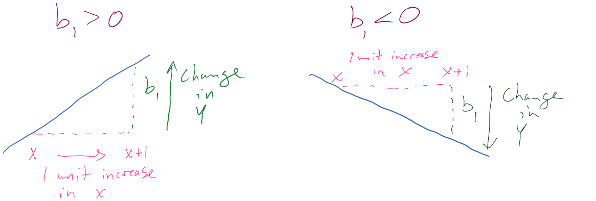
Figure 6.14: Diagram of interpretation of slope coefficients.

Figure 6.14 can help you think about the different sorts of slope coefficients we might need to interpret, both providing changes in the response variable for 1 unit increases in the predictor variable.

Applied to this problem, for each additional 1 beer consumed, we expect a 0.018 gram per dL change in the BAC on average. Using “change” in the interpretation for what happened in the response allows you to use the same template for the interpretation even with negative slopes – be careful about saying “decrease” when the slope is negative as you can create a double-negative and end up implying an increase… Note also that you need to carefully incorporate the units of \(x\) and the units of \(y\) to make the interpretation clear. For example, if the change in BAC for 1 beer increase is 0.018, then we could also modify the size of the change in \(x\) to be a 10 beer increase and then the estimated change in BAC is \(10*0.018 = 0.18\) g/dL. Both are correct as long as you are clear about the change in \(x\) you are talking about. Typically, we will just use the units used in the original variables and only change the scale of “change in \(x\)” when it provides an interpretation we are particularly interested in.

Similarly, the general interpretation for a \(y\)-intercept is:

• \(Y\)-intercept interpretation (general): For X= 0 [units of X], we expect, on average, \(\boldsymbol{b_0}\) [units of Y] in Y.

Again, applied to the BAC data set: For 0 beers for Beers consumed, we expect, on average, -0.012 g/dL BAC. The \(y\)-intercept interpretation is often less interesting than the slope interpretation but can be interesting in some situations. Here, it is predicting average BAC for Beers=0, which is a value outside the scope of the \(x\text{'s}\) (Beers was observed between 1 and 9). Prediction outside the scope of the predictor values is called extrapolation. Extrapolation is dangerous at best and misleading at worst. That said, if you are asked to interpret the \(y\)-intercept you should still interpret it, but it is also good to note if it is outside of the region where we had observations on the explanatory variable. Another example is useful for practicing how to do these interpretations.

In the Australian Athlete data, we saw a weak negative relationship between Body Fat (% body weight that is fat) and Hematocrit (% red blood cells in the blood). The scatterplot in Figure 6.15 shows just the results for the female athletes along with the regression line which has a negative slope coefficient. The estimated regression coefficients are found using the lm function:

aisR2 <- ais[-c(56,166), c("Ht","Hc","Bfat","Sex")]
m2 <- lm(Hc~Bfat, data=subset(aisR2,Sex==1)) #Results for Females 

summary(m2)

## 
## Call:
## lm(formula = Hc ~ Bfat, data = subset(aisR2, Sex == 1))
## 
## Residuals:
##     Min      1Q  Median      3Q     Max 
## -5.2399 -2.2132 -0.1061  1.8917  6.6453 
## 
## Coefficients:
##             Estimate Std. Error t value Pr(>|t|)
## (Intercept) 42.01378    0.93269  45.046   <2e-16
## Bfat        -0.08504    0.05067  -1.678   0.0965
## 
## Residual standard error: 2.598 on 97 degrees of freedom
## Multiple R-squared:  0.02822,    Adjusted R-squared:  0.0182 
## F-statistic: 2.816 on 1 and 97 DF,  p-value: 0.09653

scatterplot(Hc~Bfat, data=subset(aisR2,Sex==1), smooth=F, pch=16,
            main="Scatterplot of Body Fat vs Hematocrit for Female Athletes",
            ylab="Hc (% blood)", xlab="Body fat (% weight)")

Figure 6.15: Scatterplot of Hematocrit versus Body Fat for female athletes.

Based on these results, the estimated regression equation is \(\widehat{\text{Hc}}_i = 42.014 - 0.085\cdot\text{BodyFat}_i\) with \(b_0 = 42.014\) and \(b_1 = 0.085\). The slope coefficient interpretation is: For a one percent increase in body fat, we expect, on average, a -0.085% (blood) change in Hematocrit for Australian female athletes. For the \(y\)-intercept, the interpretation is: For a 0% body fat female athlete, we expect a Hematocrit of 42.014% on average. Again, this \(y\)-intercept involves extrapolation to a region of \(x\)’s that we did not observed. None of the athletes had body fat below 5% so we don’t know what would happen to the hematocrit of an athlete that had no body fat except that it probably would not continue to follow a linear relationship.

6.7 Least Squares Estimation

The previous results used the lm function as a “black box” to generate the estimated coefficients. The lines produced probably look reasonable but you could imagine drawing other lines that might look equally plausible. Because we are interested in explaining variation in the response variable, we want a model that in some sense minimizes the residuals \((e_i=y_i-\widehat{y}_i)\) and explains the responses as well as possible, in other words has \(y_i-\widehat{y}_i\) as small as possible. We can’t just add these \(e_i\)’s up because it would always be 0 (remember why we use the variance to measure spread from introductory statistics?). We use a similar technique in regression, we find the regression line that minimizes the squared residuals \(e^2_i=(y_i-\widehat{y}_i)^2\) over all the observations, minimizing the Sum of Squared Residuals\(\boldsymbol{=\Sigma e^2_i}\). Finding the estimated regression coefficients that minimize the sum of squared residuals is called least squares estimation and provides us a reasonable method for finding the “best” estimated regression line of all the possible choices.

For the Beers vs BAC data, Figure 6.16 shows the result of a search for the optimal slope coefficient between values of 0 and 0.03. The plot shows how the sum of the squared residuals was minimized for the value that lm returned at 0.018. The main point of this is that if any other slope coefficient was tried, it did not do as good on the least squares criterion as the least squares estimates.

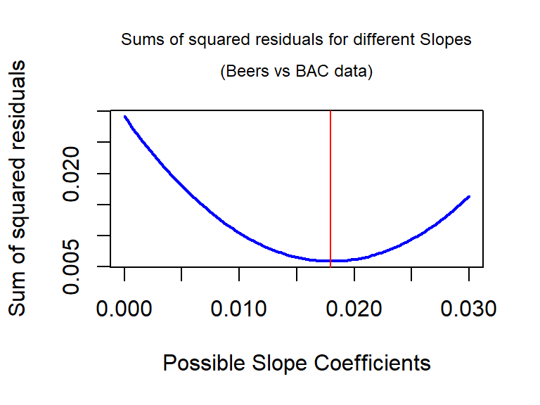
Figure 6.16: Plot of sum of squared residuals vs possible slope coefficients for Beers vs BAC data, with vertical line for the least squares estimate that minimizes the sum of squared residuals.

Sometimes it is helpful to have a go at finding the estimates yourself. If you install and load the tigerstats (Robinson and White 2016) and manipulate (Allaire 2014) packages in RStudio and then run FindRegLine(), you get a chance to try to find the optimal slope and intercept for a fake data set. Click on the “sprocket” icon in the upper left of the plot and you will see something like Figure 6.17. This interaction can help you see how the residuals are being measuring in the \(y\)-direction and appreciate that lm takes care of this for us.

> library(tigerstats)
> library(manipulate)
> FindRegLine()

Equation of the regression line is:
y = 4.34 + -0.02x

Your final score is 13143.99
Thanks for playing!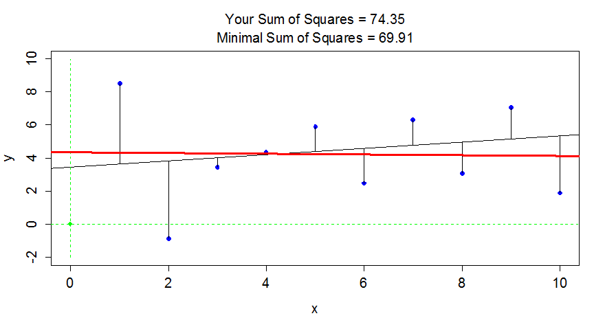

Figure 6.17: Results of running FindRegLine() where I didn’t quite find the least squares line. The correct line is the bold (red) line and produced a smaller sum of squared residuals than the guessed thinner (black) line.

It ends up that the least squares criterion does not require a search across coefficients or trial and error – there are some “simple” equations available for calculating the estimates of the \(y\)-intercept and slope:

\[b_1 = \frac{\Sigma_i(x_i-\bar{x})(y_i-\bar{y})}{\Sigma_i(x_i-\bar{x})^2} =r\frac{s_y}{s_x} \text{ and } b_0 = \bar{y} - b_1\bar{x}.\]

You will never need to use these equations but they do inform some properties of the regression line. The slope coefficient, \(b_1\), is based on the variability in \(x\) and \(y\) and the correlation between them. If \(\boldsymbol{r}=0\), then the slope coefficient will also be 0. The intercept is a function of the means of \(x\) and \(y\) and what the estimated slope coefficient is. If the slope coefficient, \(\boldsymbol{b_1}\), is 0, then \(\boldsymbol{b_0=\bar{y}}\) (which is just the mean of the response variable for all observed values of \(x\) – this is a very boring model!). The slope is 0 when the correlation is 0. So when there is no linear relationship between \(x\) and \(y\) (\(r=0\)), the least squares regression line is a horizontal line with height \(\bar{y}\), and the line produces the same fitted values for all \(x\) values. You can also think about this as when there is no relationship between \(x\) and \(y\), the best prediction of \(y\) is the mean of the \(y\)-values and it doesn’t change based on the values of \(x\). It is less obvious in these equations, but they also imply that the regression line ALWAYS goes through the point \(\boldsymbol{(\bar{x},\bar{y}).}\) It provides a sort of anchor point for all regression lines.

For one more example, we can revisit the Montana wildfire areas burned (log-hectares) and the average summer temperature (degrees F), which had \(\boldsymbol{r}=0.81\). The interpretations of the different parts of the regression model follow the least squares estimation provided by lm:

fire1 <- lm(loghectares~Temperature, data=mtfires)
summary(fire1)

## 
## Call:
## lm(formula = loghectares ~ Temperature, data = mtfires)
## 
## Residuals:
##     Min      1Q  Median      3Q     Max 
## -3.0822 -0.9549  0.1210  1.0007  2.4728 
## 
## Coefficients:
##             Estimate Std. Error t value Pr(>|t|)
## (Intercept) -69.7845    12.3132  -5.667 1.26e-05
## Temperature   1.3884     0.2165   6.412 2.35e-06
## 
## Residual standard error: 1.476 on 21 degrees of freedom
## Multiple R-squared:  0.6619, Adjusted R-squared:  0.6458 
## F-statistic: 41.12 on 1 and 21 DF,  p-value: 2.347e-06

• Regression Equation (Completely Specified):

  • Estimated model: \(\widehat{\text{log(Ha)}} = -69.78 + 1.39\cdot\text{Temp}\)

  • Or \(\widehat{y} = -69.78 + 1.39x\) with Y=log(Ha) and X=Temperature

• Response Variable: Yearly log Hectares burned by wildfires

• Explanatory Variable: Average Summer Temperature

• Estimated \(y\)-Intercept (\(b_0\)): -69.78

• Estimated slope (\(b_1\)): 1.39

• Slope Interpretation: For a 1 degree Fahrenheit increase in Average Summer Temperature we would expect, on average, a 1.39 log(Hectares) \(\underline{change}\) in log(Hectares) burned in Montana.

• \(Y\)-intercept Interpretation: If temperature were 0 degrees F, we would expect -69.78 log(Hectares) burned on average in Montana.

One other use of regression equations is for prediction. It is a trivial exercise (or maybe not – we’ll see when you try it!) to plug an \(x\)-value of interest into the regression equation and get an estimate for \(y\) at that \(x\). Basically, the regression lines displayed in the scatterplots show the predictions from the regression line across the range of \(x\text{'s}\). Formally, prediction involves estimating the response for a particular value of \(x\). We know that it won’t be perfect but it is our best guess. Suppose that we are interested in predicting the log-area burned for a summer that had an average temperature of \(59^\circ\text{F}\). If we plug \(59^\circ\text{F}\) into the regression equation, \(\widehat{\text{log(Ha)}} = -69.78 + 1.39\bullet \text{Temp}\), we get

\[\begin{array}{rl} \\ \require{cancel} \widehat{\log(\text{Ha})}&= -69.78\text{ log-hectares }+ 1.39\text{ log-hectares}/^\circ \text{F}\bullet 59^\circ\text{F} \\&= -69.78\text{ log-hectares } +1.39\text{ log-hectares}/\cancel{^\circ \text{F}}\bullet 59\cancel{^\circ \text{F}} \\&= 12.23 \text{ log-hectares} \\ \end{array}\]

We did not observe any summers at exactly \(x=59\) but did observe some nearby and this result seems relatively reasonable.

Now suppose someone asks you to use this equation for predicting \(\text{Temperature} = 65^\circ F\). We can run that through the equation: \(-69.78 + 1.39*65 = 20.57\) log-hectares. But can we trust this prediction? We did not observe any summers over 60 degrees F so we are now predicting outside the scope of our observations – performing extrapolation. Having a scatterplot in hand helps us to assess the range of values where we can reasonably use the equation – here between 54 and 60 degrees F seems reasonable.

scatterplot(loghectares~Temperature, data=mtfires, regLine=T, smooth=F, spread=F, pch=16,
            main="Scatterplot with regression line for Area burned vs Temperature")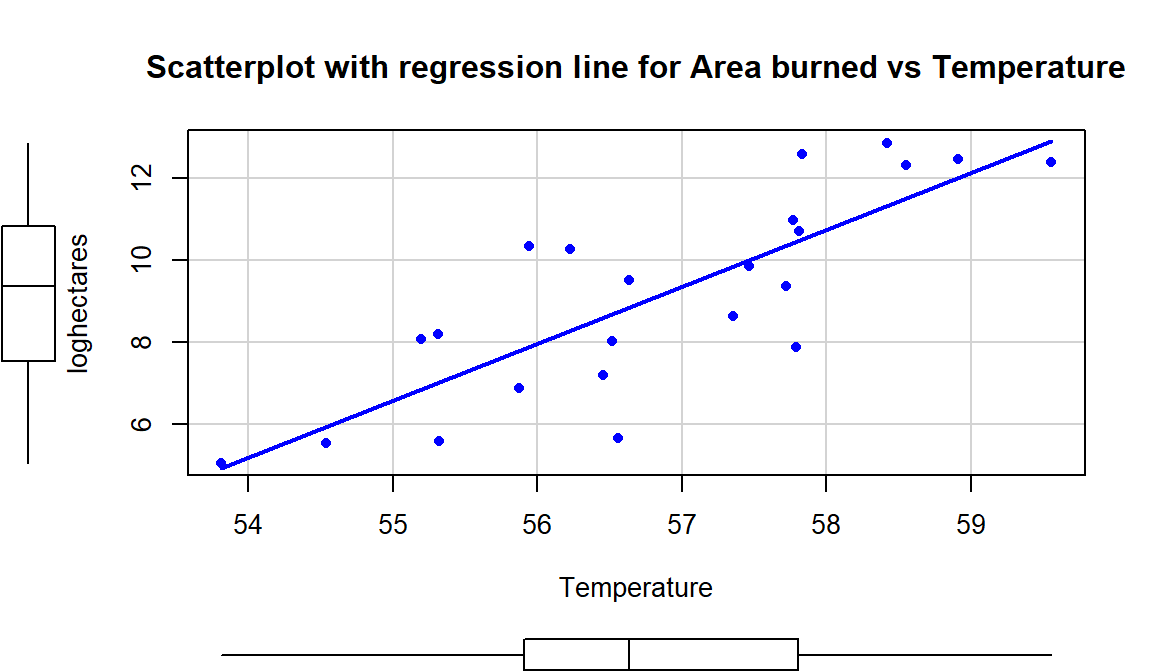

Figure 6.18: Scatterplot of log-hectares burned versus temperature with estimated regression line.

6.8 Measuring the strength of regressions: R²

At the beginning of the chapter, we used the correlation coefficient to measure the strength and direction of the linear relationship. The regression line provides an even more detailed description of the direction of the linear relationship than the correlation provided; in regression we addressed the question of “for a unit change in \(x\), what sort of change in \(y\) do we expect, on average?” whereas the correlation just addressed whether the relationship was positive or negative. However, the regression line tells us nothing about the strength of the relationship. Consider the three scatterplots in Figure 6.19: the left panel is the original BAC data and the two right panels have fake data that generated exactly the same estimated regression model with a weaker (middle panel) and then a stronger (right panel) linear relationship between Beers and BAC. This suggests that the regression line is a useful but incomplete characterization of relationships between variables – we need a measure of strength of the relationship to go with the equation.

We could use the correlation coefficient, r, again to characterize strength but it is somewhat redundant to report a measure that contains direction information. It also will not extend to multiple regression models where we have more than one predictor variable in the same model.

In regression models, we use the coefficient of determination (symbol: R²) to accompany our regression line and describe the strength of the relationship. It can either be scaled between 0 and 1 or 0 to 100% and has “units” of the proportion or percentage of the variation in \(y\) that is explained by the model that includes \(x\) (and later more than one \(x\)). For example, an R² of 0% corresponds to explaining 0% of the variation in the response with our model and \(\boldsymbol{R^2} = 100\%\) means that all the variation in the response was explained by the model. In between, it provides a nice summary of how much of the total variability in the response we can account for with our model including \(x\) (and, in Chapter 8, including multiple predictor variables).

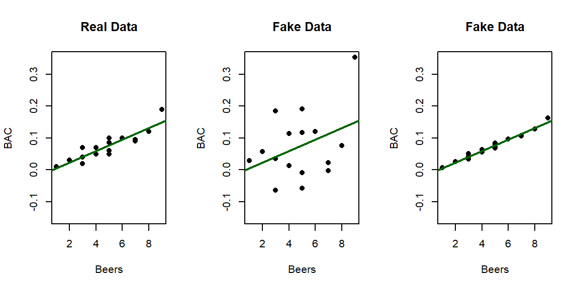
Figure 6.19: Three scatterplots with the same estimated regression line.

The R² is calculated using the sums of squares we encountered in the ANOVA methods. We once again have some total amount of variability that is attributed to the variation based on the model fit, here we call it \(\text{SS}_\text{regression}\), and the residual variability, still \(\text{SS}_\text{error}=\Sigma(y-\widehat{y})^2\). The \(\text{SS}_\text{regression}\) is most easily calculated as \(\text{SS}_\text{regression} = \text{SS}_\text{Total} - \text{SS}_\text{error}\), the difference between the total variability and the variability not explained by the model under consideration. Using these quantities, we calculate the portion of the total variability that the model explains as

\[\boldsymbol{R^2}=\frac{\text{SS}_\text{regression}}{\text{SS}_\text{Total}} =1 - \frac{\text{SS}_\text{error}}{\text{SS}_\text{Total}}.\]

It also ends up that the coefficient of determination for models with one predictor is the correlation coefficient (r) squared (\(\boldsymbol{R^2} = \boldsymbol{r^2}\)). So we can quickly find coefficients of determination if we know correlations in simple linear regression models. In the real Beers and BAC data, r=0.8943. So \(\boldsymbol{R^2} = 0.79998\) or approximately 0.80. So 80% of the variation in BAC is explained by Beer consumption. That leaves 20% of the variation in the responses to be unexplained by our model. In this case much of the unexplained variation is likely attributable to differences in physical characteristics (that were not measured) but the statistical model places that unexplained variation into the category of “random errors”. We don’t actually have to find r to get coefficients of determination – the result is part of the regular summary of a regression model that we have not discussed. We repeat the full lm model summary below – note that a number is reported for the “Multiple R-squared” in the second to last line of the output. It is reported as a proportion and it is your choice whether you want to report and interpret it as a proportion or percentage, just make that clear in how you discuss it.

m1 <- lm(BAC~Beers, data=BB)
summary(m1)

## 
## Call:
## lm(formula = BAC ~ Beers, data = BB)
## 
## Residuals:
##       Min        1Q    Median        3Q       Max 
## -0.027118 -0.017350  0.001773  0.008623  0.041027 
## 
## Coefficients:
##              Estimate Std. Error t value Pr(>|t|)
## (Intercept) -0.012701   0.012638  -1.005    0.332
## Beers        0.017964   0.002402   7.480 2.97e-06
## 
## Residual standard error: 0.02044 on 14 degrees of freedom
## Multiple R-squared:  0.7998, Adjusted R-squared:  0.7855 
## F-statistic: 55.94 on 1 and 14 DF,  p-value: 2.969e-06

In this output, be careful because there is another related quantity called Adjusted R-squared that we will discuss later. This other quantity is not a measure of the strength of the relationship but will be useful.

We could also revisit the ANOVA table for this model to verify the source of the R² of 0.80 based on \(\text{SS}_\text{regression}= 0.02337\) and \(\text{SS}_\text{Total} = 0.02337+0.00585\). This provides 0.80 from \(0.02337/0.02922\).

anova(m1)

## Analysis of Variance Table
## 
## Response: BAC
##           Df    Sum Sq   Mean Sq F value    Pr(>F)
## Beers      1 0.0233753 0.0233753  55.944 2.969e-06
## Residuals 14 0.0058497 0.0004178

SStotal <- 0.0233753 + 0.0058497
SSregression <- 0.0233753
SSregression/SStotal

## [1] 0.7998392

In Figure 6.19, there are three examples with the same regression model, but different strengths of relationships. In the real data set \(\boldsymbol{R^2} = 80\%\). For the first fake data set (middle panel), the R² drops to \(13.8\%\) and for the second fake data set (right panel), R² is \(97.3\%\). As a summary, R² provides a natural scale to understand “how good” each model is at explaining the responses. We can revisit some of our previous models to get a little more practice with using this summary of strength or quality of regression models.

For the Montana fire data, \(\boldsymbol{R^2}=66.2\%\). So the proportion of variation of log-area burned that is explained by average summer temperature is 0.662. This is “good” but also leaves quite a bit of unexplained variation in the responses. There is a long list of reasons why this explanatory variable leaves a lot of variation in the response unexplained. Note that we were careful about using the scaling of the response variable (log(area burned)) in the interpretation – this is because we would get a much different answer if area burned vs temperature was considered.

fire1 <- lm(loghectares~Temperature, data=mtfires)
summary(fire1)

## 
## Call:
## lm(formula = loghectares ~ Temperature, data = mtfires)
## 
## Residuals:
##     Min      1Q  Median      3Q     Max 
## -3.0822 -0.9549  0.1210  1.0007  2.4728 
## 
## Coefficients:
##             Estimate Std. Error t value Pr(>|t|)
## (Intercept) -69.7845    12.3132  -5.667 1.26e-05
## Temperature   1.3884     0.2165   6.412 2.35e-06
## 
## Residual standard error: 1.476 on 21 degrees of freedom
## Multiple R-squared:  0.6619, Adjusted R-squared:  0.6458 
## F-statistic: 41.12 on 1 and 21 DF,  p-value: 2.347e-06

For the model for female Australian athletes that used Body fat to explain Hematocrit, the estimated regression model was \(\widehat{\text{Hc}}_i = 42.014 - 0.085\cdot\text{BodyFat}_i\) and \(\boldsymbol{r} = -0.168\). The coefficient of determination is \(\boldsymbol{R^2} = (-0.168)^2 = 0.0282\). So body fat explains 2.8% of the variation in Hematocrit in these women. That is not a very good regression model with over 97% of the variation in Hematocrit unexplained by this model. The scatterplot showed a fairly weak relationship but this provides numerical and interpretable information that drives that point home.

m2 <- lm(Hc~Bfat, data=subset(aisR2,Sex==1)) #Results for Females
summary(m2)

## 
## Call:
## lm(formula = Hc ~ Bfat, data = subset(aisR2, Sex == 1))
## 
## Residuals:
##     Min      1Q  Median      3Q     Max 
## -5.2399 -2.2132 -0.1061  1.8917  6.6453 
## 
## Coefficients:
##             Estimate Std. Error t value Pr(>|t|)
## (Intercept) 42.01378    0.93269  45.046   <2e-16
## Bfat        -0.08504    0.05067  -1.678   0.0965
## 
## Residual standard error: 2.598 on 97 degrees of freedom
## Multiple R-squared:  0.02822,    Adjusted R-squared:  0.0182 
## F-statistic: 2.816 on 1 and 97 DF,  p-value: 0.09653

6.9 Outliers: leverage and influence

In the review of correlation, we loosely considered the impacts of outliers on the correlation. We removed unusual points to see both the visual changes (in the scatterplot) as well as changes in the correlation coefficient in Figures 6.4 and 6.5. In this section, we formalize these ideas in the context of impacts of unusual points on our regression equation. In regression, it is possible for a single point to have a big impact on the overall regression results but it is also possible to have a clear outlier that has little impact on the results. We call an observation influential if its removal causes a “big” change in the regression line, specifically in terms of impacting the slope coefficient. Points that are on the edges of the \(x\text{'s}\) (far from the mean of the \(x\text{'s}\)) have the potential for more impact on the line as we will see in some examples shortly.

You can think of the regression line being balanced at \(\bar{x}\) and the further from that location a point is, the more a single point can move the line. We can measure the distance of points from \(\bar{x}\) to quantify each observation’s potential for impact on the line using what is called the leverage of a point. Leverage is a positive numerical measure with larger values corresponding to more leverage. The scale changes depending on the sample size (\(n\)) and the complexity of the model so all that matters is which observations have more or less relative leverage in a particular data set. The observations with \(x\)-values that provide higher leverage have increased potential to influence the estimated regression line. Along with measuring the leverage, we can also measure the influence that each point has on the regression line using Cook’s Distance or Cook’s D. It also is a positive measure with higher values suggesting more influence. The rule of thumb is that Cook’s D values over 1.0 correspond to clearly influential points, values over 0.5 have some influence and values lower than 0.5 indicate points that are not influential on the regression model slope coefficients. One part of the regular diagnostic plots we will use for regression models displays the leverages on the \(x\)-axis, the standardized residuals on the \(y\)-axis, and adds contour lines for Cook’s Distances in a panel that is labeled “Residuals vs Leverage”. This allows us to see the potential for impact of a point (leverage), how far it’s observation was from the regression line (residual), and to see a measure of that point’s influence (Cook’s D).

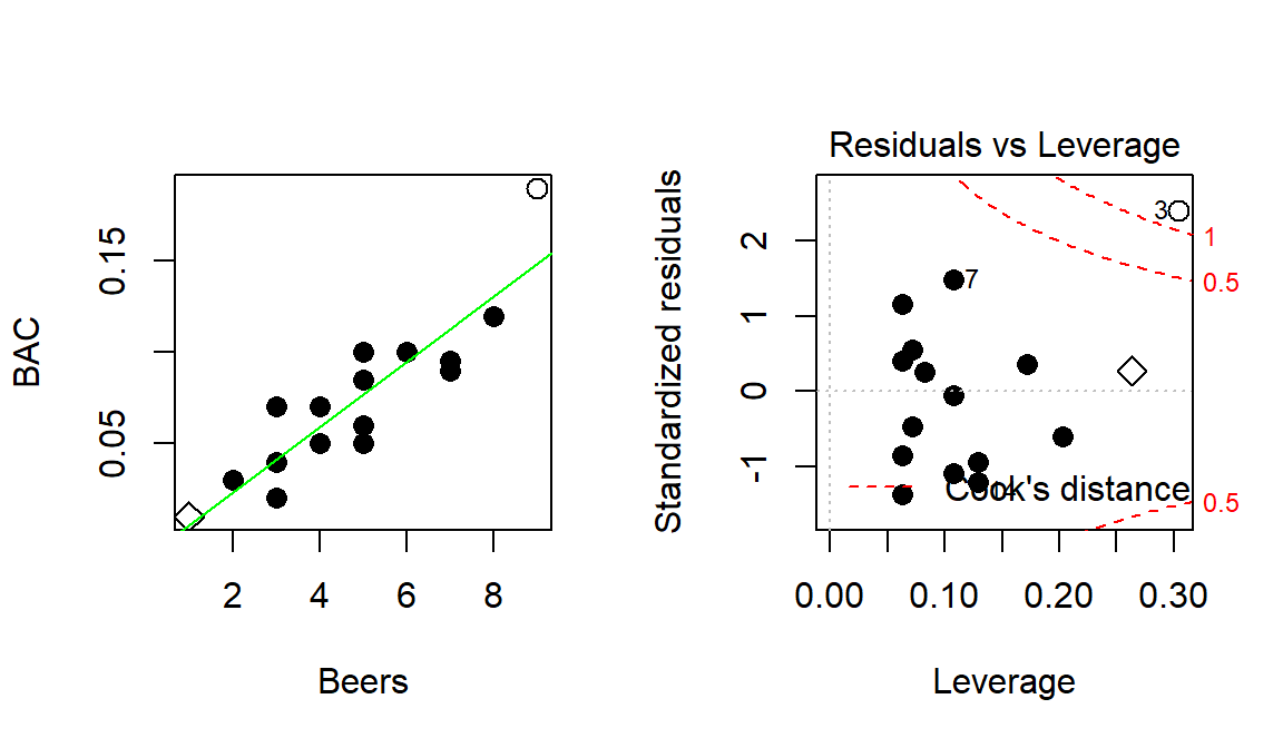
Figure 6.20: Scatterplot and Residuals vs Leverage plot for the real BAC data. Two high leverage points are flagged, with only one that has a Cook’s D value over 1 (“\(\circ\)”) and is indicated as influential.

To extract the level of Cook’s D on the “Residuals vs Leverage” plot, look for contours to show up on the upper and lower right of the plot. They show increasing levels of influence going to the upper and lower right corners as you combine higher leverage (\(x\)-axis) and larger residuals (\(y\)-axis) – the two ingredients required to be influential on the line. The contours are displayed for Cook’s D values of 0.5 and 1.0 if there are points near or over those levels. The Cook’s D values come from a topographical surface of values that is a sort of U-shaped valley in the middle of the plot centered at \(y=0\) with the lowest contour corresponding to Cook’s D values below 0.5 (no influence). As you move to the upper right or lower right corners, the influence increases and the edges of the valley get steeper. If you do not see any contours in the plot, then no points were even close to being influential based on Cook’s D.

To illustrate these concepts, the original Beers and BAC data are used again. In the scatter plot in Figure 6.20, two points are plotted with different characters. The point for 1 Beer and BAC of 0.010 is displayed as a “\(\diamond\)” and the 9 Beer and BAC 0.19 observation is displayed with a “\(\circ\)”. These two points are the furthest from the mean of the of the \(x\text{'s}\) (\(\overline{\text{Beers}}= 4.8\)) but show two different levels of influence on the line. The “\(\diamond\)” point has a leverage of 0.27 and the 9 Beer observation (“\(\circ\)”) had a leverage of 0.30. The 1 Beer observation was close to the pattern defined by the other points, had a small residual, and a Cook’s D value below 0.5 (it did not exceed the first of the contours). So even though it had high leverage, it was not an influential point. The 9 Beer observation had the highest leverage in the data set and was quite a bit above the pattern defined by the other points and ends up being an influential point with a Cook’s D over 1. We might want to consider fitting this model without that observation to get a better estimate of the effects of beer consumption on BAC or revisit our assumption that the relationship is really linear here.

To further explore influence, we will add a point to the original data set and move it around so you can see how those changes impact the results. For each scatterplot in Figure 6.21, the Residuals vs Leverage plot is displayed to its right. The original data are “\(\color{Grey}{\bullet}\)” and the original regression line is the dashed line in Figure 6.21. First, a fake observation at 11 Beers and 0.1 BAC is added, at (11, 0.1), in the top panels of the figure. This observation is clearly an outlier and heavily impacts the slope of the regression line (so is clearly influential). This added point drops the R² from 0.80 in the original data to 0.24. The accompanying Residuals vs Leverage plot shows that this point has extremely high leverage and a Cook’s D over 1 – it is a clearly influential point. However, having high leverage does not always make points influential. Consider the second row of plots with an added point of (11, 0.19). The regression line barely changes and R² increases a little. This point has the same leverage as in the first example since it is the same set of \(x\text{'s}\) and the distance to the mean of the \(x\)’s is unchanged. But it is not influential since its Cook’s D value is less than 0.5. This occurred because it followed the overall pattern of observations even though it was “far away” from the other observations in the \(x\)-direction. The last two rows of plots show what happens when low leverage outliers are encountered. If observations are near the center of the \(x\text{'s}\), it ends up that to be influential the points have to be very far from the pattern of the other observations. The (5, 0.19) example almost attains a Cook’s D of 0.5 but has little impact on the regression line, especially the slope coefficient. It does impact the \(y\)-intercept and drops the R-squared value to 0.57. The same result occurs if the observation is noticeably lower than the other points.

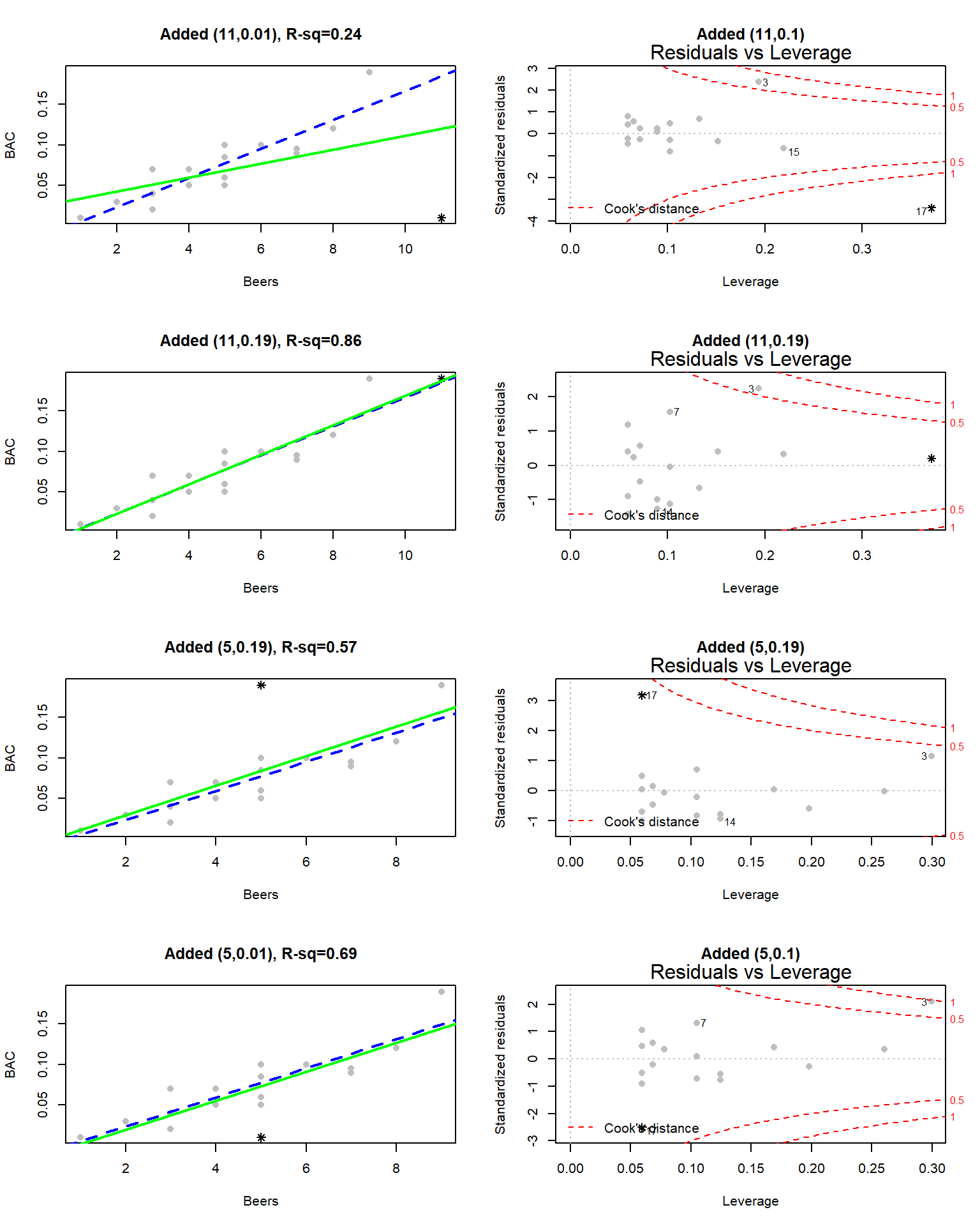
Figure 6.21: Plots exploring the impacts of moving a single additional observation in the BAC example. The added point is indicated with * and the original regression line is the dashed line in the left column.

When we are doing regressions, we get very worried about points “at the edges” having an undue influence on the results. When we start using multiple predictors, say if we had body weight data on these subjects as well as beer consumption, it becomes harder to “see” if the points are “far away” from the other observations and we will trust the Residuals vs Leverage plots to help us identify the influential points. These techniques work the same in the multiple regression models in Chapter 8 as they do in these simpler, single predictor regression models.

6.10 Residual diagnostics – setting the stage for inference

Influential points are not the only potential issue that can cause us to have concerns about our regression model. There are two levels to these considerations. The first is related to issues that directly impact the least squares regression line and cause concerns about whether a line is a reasonable representation of the relationship between the two variables. These issues for regression model estimation have been discussed previously (the same concerns in estimating correlation apply to regression models). The second level is whether the line we have will be useful for making inferences for the population that our data were collected from and whether the data follow our assumed model. Our window into problems of both types is the residuals \((e_i = y_i - \widehat{y}_i)\). By exploring patterns in how the line “misses” the responses we can gain information about the reasonableness of using the estimated regression line and sometimes information about how we might fix problems. The validity conditions for doing inference in a regression setting (Chapter 7) involve two sets of considerations, those that are assessed based on the data collection and measurement process and those that can be assessed using diagnostic plots. The first set is:

• Quantitative variables condition

  • We’ll discuss using categorical predictor variables later – to use simple linear regression both the explanatory and response variables need to quantitative.

• Independence of observations

  • As in the ANOVA models, linear regression models assume that the observations are collected in a fashion that makes them independent.

  • This will be based on the “story” of the data. Consult a statistician if your data violate this assumption as there are more advanced methods that adjust for dependency in observations but they are beyond the scope of this material.

The remaining assumptions for getting valid inferences from regression models can be assessed using diagnostic plots:

• Linearity of relationship

  • We should not report a linear regression model if the data show a curve (curvilinear relationship between \(x\) and \(y\)).

  • Examine the initial scatterplot to assess the potential for a curving relationship.

  • Examine the Residuals vs Fitted (top left panel of diagnostic plot display) plot:

    • If the model missed a curve in the relationship, the residuals often will highlight that missed pattern and a curve will show up in this plot.

    • Try to explain or understand the pattern in what is left over. If we have a good model, there shouldn’t be much left to “explain” in the residuals (i.e., no patterns left over after accounting for \(x\)).

• Equal (constant) variance

  • We assume that the variation is the same for all the observations and especially that the variability does not change in the responses as a function of our predictor variables or the fitted values.

  • There are three plots to help with this:

    • Examine the original scatterplot and look at the variation around the line and whether it looks constant across values of \(x\).

    • Examine the Residuals vs Fitted plot and look for evidence of changing spread in the residuals, being careful to try to separate curving patterns from non-constant variance (and look for situations where both are present as you can violate both conditions simultaneously).

    • Examine the “Scale-Location” plot and look for changing spread as a function of the fitted values.

      • The \(y\)-axis in this plot is the square-root of the absolute value of the standardized residual. This scale flips the negative residuals on top of the positive ones to help you better assess changing variability without being distracted by whether the residuals are above or below 0.

      • Because of the absolute value, curves in the Residuals vs Fitted plot can present as sort of looking like non-constant variance in the Scale-Location plot – check for nonlinearity in the residuals vs fitted values before using this plot. If nonlinearity is present, just use the Residuals vs Fitted and original scatterplot for assessing constant variance around the curving pattern.

  • If there are patterns of increasing or decreasing variation (often described as funnel or cone shapes), then it might be possible to use a transformation to fix this problem (more later). It is possible to have decreasing and then increasing variability and this also is a violation of this condition.

• Normality of residuals

  • Examine the Normal QQ-plot for violations of the normality assumption as in Chapters 3 and 4.

    • Specifically review the discussion of identifying skews in different directions and heavy vs light tailed distributions.

    • Skewed and heavy-tailed distributions are the main problems for our inferences, especially since both kinds of distributions can contain outliers that can wreak havoc on the estimated regression line.

    • Light-tailed distributions cause us no real inference issues except that the results are conservative so you should note when you observe these situations but feel free to proceed with using your model results.

    • Remember that clear outliers are an example of a violation of the normality assumption but some outliers may just influence the regression line and make it fit poorly and this issue will be more clearly observed in the residuals vs fitted than in the QQ-plot.

• No influential points

  • Examine the Residuals vs Leverage plot as discussed in the previous section.

  • Consider removing influential points (one at a time) and focusing on results without those points in the data set.

To assess these later assumptions, we will use the four residual diagnostic plots that R provides from lm fitted models. They are similar to the results from ANOVA models but the Residuals vs Leverage plot is now interesting as was discussed in Section 6.9. Now we can fully assess the potential for trusting the estimated regression models in a couple of our examples:

• Beers vs BAC:

  • Quantitative variables condition:

    • Both variables are quantitative.

  • Independence of observations:

    • We can assume that all the subjects are independent of each other. There is only one measurement per student and it is unlikely that one subject’s beer consumption would impact another’s BAC. Unless the students were trading blood it isn’t possible for one person’s beer consumption to change someone else’s BAC.

    m1 <- lm(BAC~Beers, data=BB)
    par(mfrow=c(2,2))
    plot(m1, add.smooth=F, main="Beers vs BAC", pch=16)

    

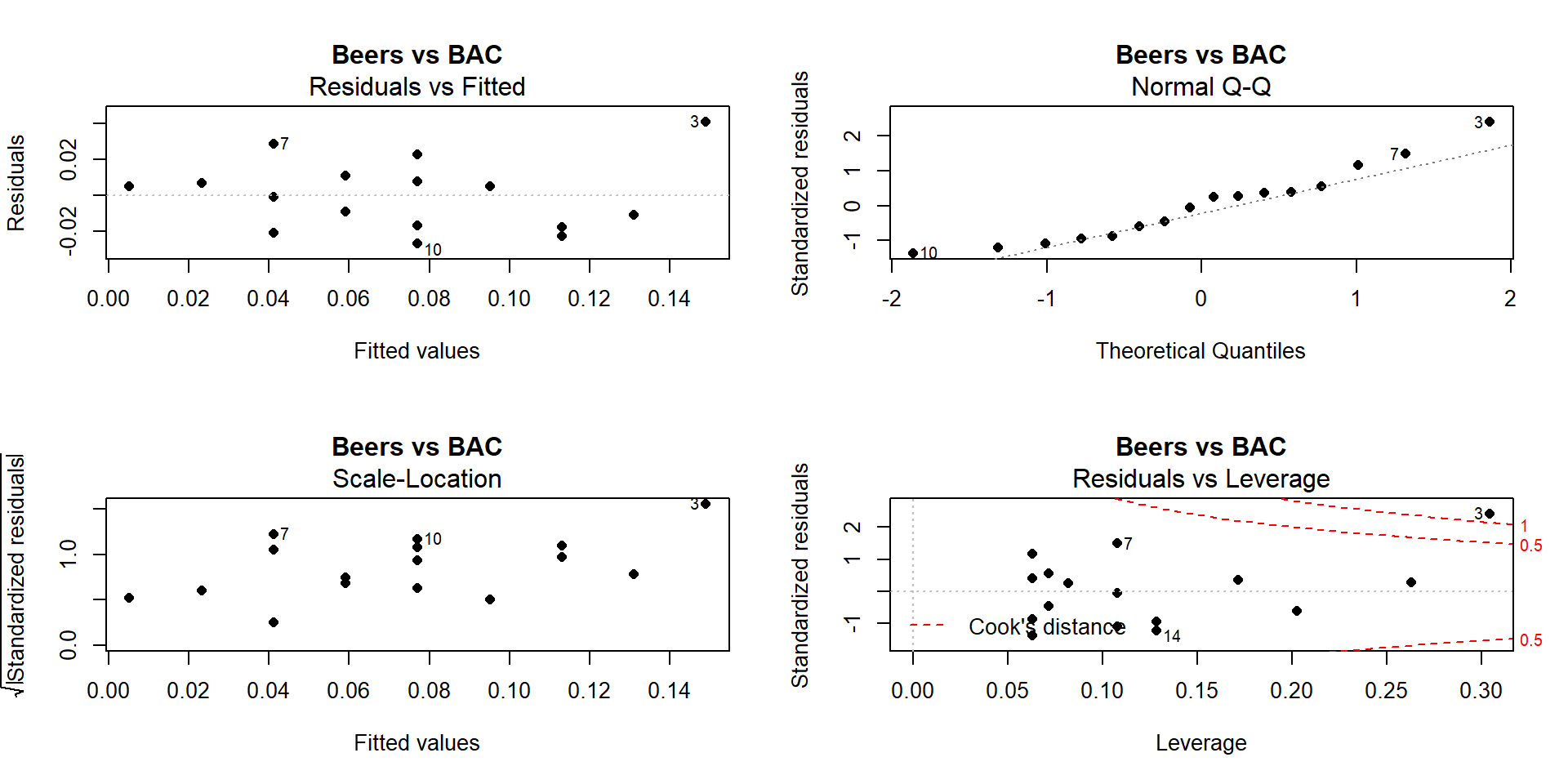
    Figure 6.22: Full suite of diagnostics plots for Beer vs BAC data.

  • Linearity, constant variance from Residuals vs Fitted:

    • We previously have identified a potentially influential outlier point in these data. Consulting the Residuals vs Fitted plot in Figure 6.22, if you trust that influential point, shows some curvature with a pattern of decreasing residuals as a function of the fitted values and then an increase at the right. Or, if you do not trust that highest BAC observation, then there is a mostly linear relationship with an outlier identified. We would probably suggest that it is an outlier, should be removed from the analysis, and inferences constrained to the region of beer consumption from 1 to 8 beers since we don’t know what might happen at higher values.

  • Constant variance from Scale-Location:

    • There is some evidence of increasing variability in this plot as the spread of the results increases from left to right, however this is just an artifact of the pattern in the original residuals and not real evidence of non-constant variance. Note that there is little to no evidence of non-constant variance in the Residuals vs Fitted.

  • Normality from Normal QQ Plot:

    • The left tail is a little short and the right tail is a little long, suggesting a slightly right skewed distribution in the residuals. This also corresponds to having a large positive outlying value. But we would conclude that there is a minor issue with normality in the residuals here.

  • Influential points from Residuals vs Leverage:

    • Previously discussed, this plot shows one influential point with a Cook’s D value over 1 that is distorting the fitted model and is likely the biggest issue here.

• Tree height and tree diameter (suspicious observation already removed):

  • Quantitative variables: Met

  • Independence of observations:

    • There are multiple trees that were measured in each plot. One problem might be that once a tree is established in an area, the other trees might not grow as tall. The other problem is that some sites might have better soil conditions than others. Then, all the trees in those rich soil areas might be systematically taller than the trees in other areas. Again, there are statistical methods to account for this sort of “clustering” of measurements but this technically violates the assumption that the trees are independent of each other. So this assumption is violated, but we will proceed with that caveat on our results – the precision of our inferences might be slightly over-stated due to some potential dependency in the measurements.

  • Linearity, constant variance from Residuals vs Fitted in Figure 6.23.

    • There is evidence of a curve that was missed by the linear model.

    • There is also evidence of increasing variability AROUND the curve in the residuals.

  • Constant variance from Scale-Location:

    • This plot actually shows relatively constant variance but this plot is misleading when curves are present in the data set. Focus on the Residuals vs Fitted to diagnose non-constant variance in situations where a curve was missed.

  • Normality in Normal QQ plot:

    • There is no indication of any problem with the normality assumption.

  • Influential points?

    • The Cook’s D contours do not show up in this plot so none of the points are influential.

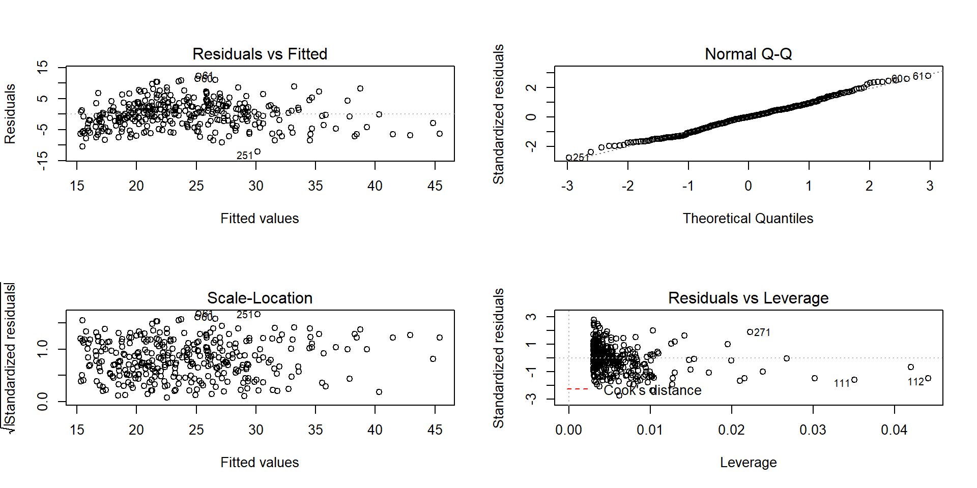
Figure 6.23: Diagnostics plots for tree height and diameter simple linear regression model.

So the main issues with this model are the curving relationship and non-constant variance. We’ll revisit this example later to see if we can find a model on transformed variables that has better diagnostics. Reporting the following regression model that has a decent \(R^2\) of 62.6% would be misleading since it does not accurately represent the relationship between tree diameter and tree height.

tree1 <- lm(height.m~dbh.cm, data=ufc[-168,])
summary(tree1)

## 
## Call:
## lm(formula = height.m ~ dbh.cm, data = ufc[-168, ])
## 
## Residuals:
##      Min       1Q   Median       3Q      Max 
## -12.1333  -3.1154   0.0711   2.7548  12.3076 
## 
## Coefficients:
##             Estimate Std. Error t value Pr(>|t|)
## (Intercept) 11.98364    0.57422   20.87   <2e-16
## dbh.cm       0.32939    0.01395   23.61   <2e-16
## 
## Residual standard error: 4.413 on 333 degrees of freedom
## Multiple R-squared:  0.626,  Adjusted R-squared:  0.6249 
## F-statistic: 557.4 on 1 and 333 DF,  p-value: < 2.2e-16

par(mfrow=c(2,2))
plot(tree1, add.smooth=F)

6.11 Old Faithful discharge and waiting times

A study in August 1985 considered time for Old Faithful and how that might relate to waiting time for the next eruption (Ripley (2019), Azzalini and Bowman (1990)). This sort of research provides the Yellowstone National Park (YNP) staff a way to show tourists a predicted time to next eruption so they can quickly see it erupt and then get back in their cars, not wasting too much time in the outdoors. Or, less cynically, the opportunity to study the behavior of the eruption of a geyser. Both variables are measured in minutes and the scatterplot in Figure 6.24 shows a moderate to strong positive and relatively linear relationship. We added a smoothing line (dashed line) to this plot. Smoothing lines provide regression-like fits but are performed on local areas of the relationship between the two variables and so can highlight where the relationships change, especially highlighting curvilinear relationships. They can also return straight lines just like the regression line if that is reasonable. The technical details of regression smoothing are not covered here but they are a useful graphical addition to help visualize nonlinearity in relationships.

In these data, there appear to be two groups of eruptions (shorter length, shorter wait and longer length, longer wait) – but we don’t know enough about these data to assume that there are two groups. The smoothing line does help us to see if the relationship appears to change or stay the same across different values of the explanatory variable, Duration. The smoothing line suggests that the upper group might have a less steep slope than the lower group as it sort of levels off for observations with Duration of over 4 minutes. It also indicates that there is one point for an eruption under 1 minute in Duration that might be causing some problems. The story of these data involve some measurements during the night that were just noted as being short, medium, and long – and they were re-coded as 2, 3, or 4 minute duration eruptions. You can see responses stacking up at 2 and 4 minute durations and this is obviously a problematic aspect of these data. We’ll see if our diagnostics detect some of these issues when we fit a simple linear regression to try to explain waiting time based on duration of prior eruption.

library(MASS)
data(geyser)
geyser <- as_tibble(geyser)
#Aligns the duration with time to next eruption
G2 <- tibble(Waiting=geyser$waiting[-1], Duration=geyser$duration[-299]) 
scatterplot(Waiting~Duration, data=G2, smooth=list(spread=F)) #Adds smoothing line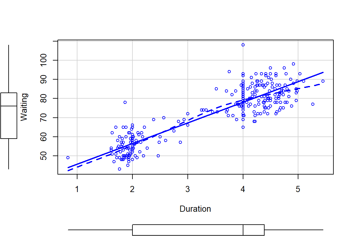

Figure 6.24: Scatterplot of Old Faithful waiting times to next eruption (minutes) and duration of prior eruption (minutes) with smoothing line (dashed) and regression line (solid).

An initial concern with these data is that the observations are likely not independent. Since they were taken consecutively, one waiting time might be related to the next waiting time – violating the independence assumption. As noted above, there might be two groups (types) of eruptions – short ones and long ones. The Normal QQ-Plot in Figure 6.25 also suggests a few observations creating a slightly long right tail. Those observations might warrant further exploration as they also show up as unusual in the Residuals vs Fitted plot. There are no highly influential points in the data set with all points having Cook’s D smaller than 0.5 (contours are not displayed because no points are near or over them), so these outliers are not necessarily moving the regression line around. There are two distinct groups of observations but the variability is not clearly changing so we do not have to worry about non-constant variance here. So these results might be relatively trustworthy if we assume that the same relationship holds for all levels of duration of eruptions.

OF1 <- lm(Waiting~Duration, data=G2)

summary(OF1)

## 
## Call:
## lm(formula = Waiting ~ Duration, data = G2)
## 
## Residuals:
##      Min       1Q   Median       3Q      Max 
## -14.6940  -4.4954  -0.0966   3.9544  29.9544 
## 
## Coefficients:
##             Estimate Std. Error t value Pr(>|t|)
## (Intercept)  34.9452     1.1807   29.60   <2e-16
## Duration     10.7751     0.3235   33.31   <2e-16
## 
## Residual standard error: 6.392 on 296 degrees of freedom
## Multiple R-squared:  0.7894, Adjusted R-squared:  0.7887 
## F-statistic:  1110 on 1 and 296 DF,  p-value: < 2.2e-16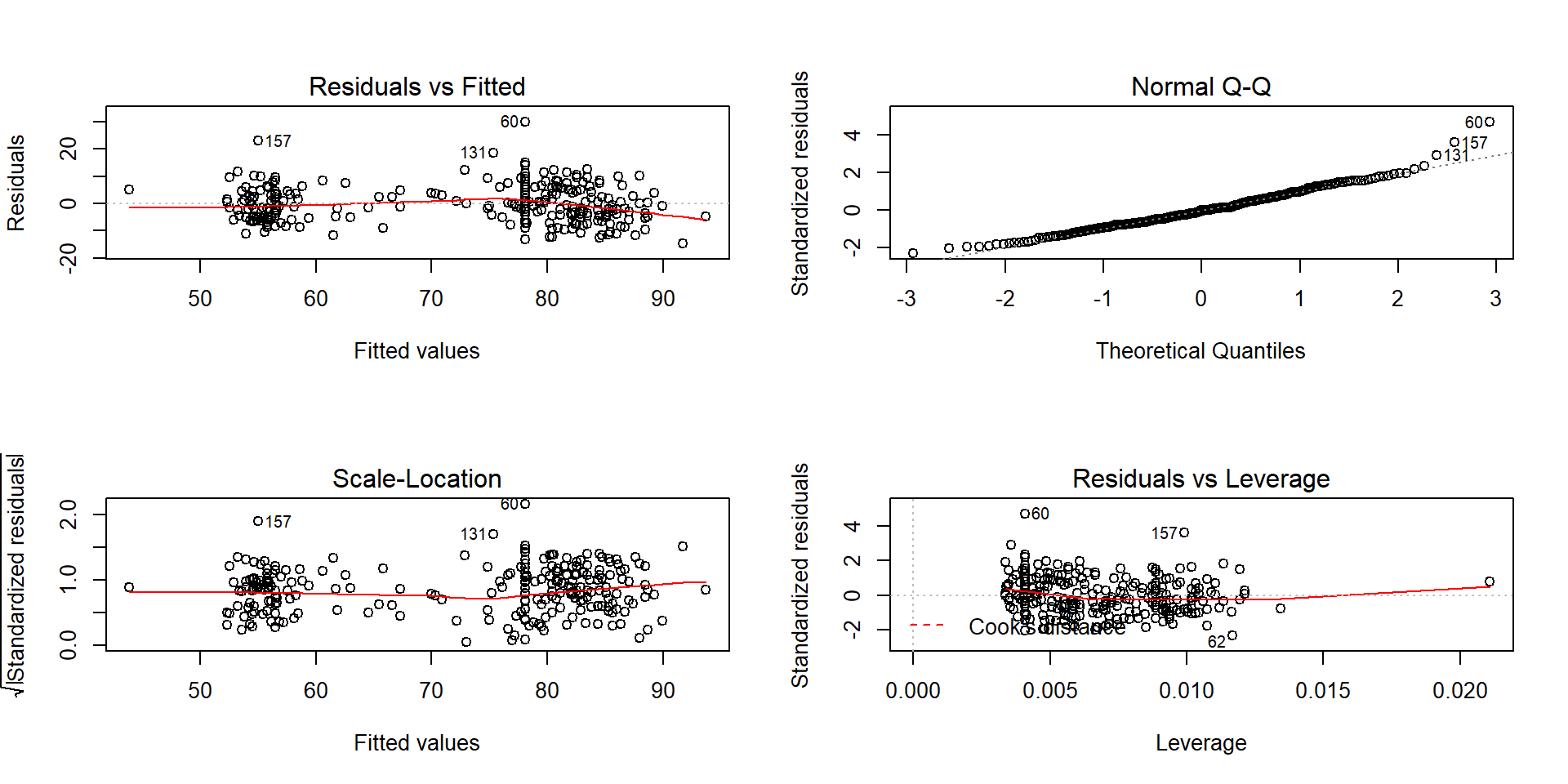

par(mfrow=c(2,2))
plot(OF1)

Figure 6.25: Diagnostic plots for Old Faithful waiting time model.

The estimated regression equation is \(\widehat{\text{WaitingTime}}_i = 34.95 + 10.78\cdot\text{Duration}_i\), suggesting that for a 1 minute increase in eruption Duration we would expect, on average, a 10.78 minute change in the WaitingTime. This equation might provide a useful tool for the YNP staff to predict waiting times. The R² is fairly large: 78.9% of the variation in waiting time is explained by the duration of the previous eruption. But maybe this is more about two types of eruptions/waiting times? We could consider the relationship within the shorter and longer eruptions but since there are observations residing between the two groups, it is difficult to know where to split the explanatory variable into two groups. Maybe we really need to measure additional information that might explain why there are two groups in the responses…

6.12 Chapter summary

The correlation coefficient (\(\boldsymbol{r}\) or Pearson’s Product Moment Correlation Coefficient) measures the strength and direction of the linear relationship between two quantitative variables. Regression models estimate the impacts of changes in \(x\) on the mean of the response variable \(y\). Direction of the assumed relationship (which variable explains or causes the other) matters for regression models but does not matter for correlation. Regression lines only describe the pattern of the relationship; in regression, we use the coefficient of determination to describe the strength of the relationship between the variables as a percentage of the response variable that is explained by the model. If we are choosing between models, we prefer them to have higher \(R^2\) values for obvious reasons, but we will discover in Chapter 8 that maximizing the coefficient of determination is not a good way to pick a model when we have multiple candidate options.

In this chapter, a wide variety of potential problems were explored when using regression models. This included a discussion of the conditions that will be required for using the models to perform trustworthy inferences in the remaining chapters. It is important to remember that correlation and regression models only measure the linear association between variables and that can be misleading if a nonlinear relationship is present. Similarly, influential observations can completely distort the apparent relationship between variables and should be assessed before trusting any regression output. It is also important to remember that regression lines should not be used outside the scope of the original observations – extrapolation should be checked for and avoided whenever possible or at least acknowledged when it is being performed.

Regression models look like they estimate the changes in \(y\) that are caused by changes in \(x\), especially when you use \(x\) to predict \(y\). This is not true unless the levels of \(x\) are randomly assigned and only then we can make causal inferences. Since this is not generally true, you should initially always assume that any regression equation describes the relationship – if you observe two subjects that are 1 unit of \(x\) apart, you can expect their mean to differ by \(b_1\) – you should not, however, say that changing \(x\) causes a change in the mean of the responses. Despite all these cautions, regression models are very popular statistical methods. They provide detailed descriptions of relationships between variables and can be extended to situations where we are interested in multiple predictor variables. They also share ties to the ANOVA models discussed previously. When you are running R code, you will note that all the ANOVAs and the regression models are estimated using lm. The assumptions and diagnostic plots are quite similar. And in the next chapter, we will see that inference techniques look similar. People still like to distinguish among the different types of situations, but the underlying linear models are actually exactly the same…

6.13 Summary of important R code

The main components of the R code used in this chapter follow with the components to modify in lighter and/or ALL CAPS text where y is a response variable, x is an explanatory variable, and the data are in DATASETNAME.

• pairs.panels(DATASETNAME, ellipses=F, scale=T, smooth=F, col=0)

  • Requires the psych package.

  • Makes a scatterplot matrix that also displays the correlation coefficient.

• cor(y~x, data=DATASETNAME)

  • Provides the estimated correlation coefficient between \(x\) and \(y\).

• plot(y~x, data=DATASETNAME)

  • Provides a scatter plot.

• scatterplot(y~x, data=DATASETNAME, smooth=F)

  • Requires the car package.

  • Provides a scatter plot with a regression line.

• MODELNAME <- lm(y~x, data=DATASETNAME)

  • Estimates a regression model using least squares.

• summary(MODELNAME)

  • Provides parameter estimates and R-squared (used heavily in Chapter 7 and 8 as well).

• par(mfrow=c(2, 2)); plot(MODELNAME)

  • Provides four regression diagnostic plots in one plot.

6.14 Practice problems

6.1. Treadmill data analysis These questions revisit the treadmill data set from Chapter 1. Researchers were interested in whether the run test variable could be used to replace the treadmill oxygen consumption variable that is expensive to measure. The following code loads the data set and provides a scatterplot matrix using pairs.panel.

treadmill <- read_csv("http://www.math.montana.edu/courses/s217/documents/treadmill.csv")
library(psych)
pairs.panels(treadmill, ellipses=F, smooth=F, col=0)

6.1.1. First, we should get a sense of the strength of the correlation between the variable of primary interest, TreadMillOx, and the other variables and consider whether outliers or nonlinearity are going to be major issues here. Which variable is it most strongly correlated with? Which variables are next most strongly correlated with this variable?

6.1.2. Fit the SLR using RunTime as explanatory variable for TreadMillOx. Report the estimated model.

6.1.3. Predict the treadmill oxygen value for a subject with a run time of 14 minutes. Repeat for a subject with a run time of 16 minutes. Is there something different about these two predictions?

6.1.4. Interpret the slope coefficient from the estimated model, remembering the units on the variables.

6.1.5. Report and interpret the \(y\)-intercept from the SLR.

6.1.6. Report and interpret the \(R^2\) value from the output. Show how you can find this value from the original correlation matrix result.

6.1.7. Produce the diagnostic plots and discuss any potential issues. What is the approximate leverage of the highest leverage observation and how large is its Cook’s D? What does that tell you about its potential influence in this model?

References

Allaire, JJ. 2014. Manipulate: Interactive Plots for Rstudio. https://CRAN.R-project.org/package=manipulate.

Azzalini, Adelchi, and Adrian W. Bowman. 1990. “A Look at Some Data on the Old Faithful Geyser.” Applied Statistics 39: 357–65.

Clevenger, Anthony P, and Nigel Waltho. 2005. “Performance Indices to Identify Attributes of Highway Crossing Structures Facilitating Movement of Large Mammals.” Biological Conservation 121 (3): 453–64.

Fox, John, and Sanford Weisberg. 2011. An R-Companion to Applied Regression, Second Edition. Thousand Oaks, CA: SAGE Publications. http://socserv.socsci.mcmaster.ca/jfox/Books/Companion.

Fox, John, Sanford Weisberg, and Brad Price. 2018. CarData: Companion to Applied Regression Data Sets. https://CRAN.R-project.org/package=carData.

Gude, Patricia H., J. Anthony Cookson, Mark C. Greenwood, and Mark Haggerty. 2009. “Homes in Wildfire-Prone Areas: An Empirical Analysis of Wildfire Suppression Costs and Climate Change.” www.headwaterseconomics.org.

Jones, Owen, Robert Maillardet, Andrew Robinson, Olga Borovkova, and Steven Carnie. 2018. SpuRs: Functions and Datasets for "Introduction to Scientific Programming and Simulation Using R". https://CRAN.R-project.org/package=spuRs.

Revelle, William. 2019. Psych: Procedures for Psychological, Psychometric, and Personality Research. https://CRAN.R-project.org/package=psych.

Ripley, Brian. 2019. MASS: Support Functions and Datasets for Venables and Ripley’s Mass. https://CRAN.R-project.org/package=MASS.

Robinson, Rebekah, and Homer White. 2016. Tigerstats: R Functions for Elementary Statistics. https://CRAN.R-project.org/package=tigerstats.

Wei, Taiyun, and Viliam Simko. 2017. Corrplot: Visualization of a Correlation Matrix. https://CRAN.R-project.org/package=corrplot.

Weisberg, Sanford. 2005. Applied Linear Regression, Third Edition. Hoboken, NJ: Wiley.

Weisberg, Sanford. 2018. Alr3: Data to Accompany Applied Linear Regression 3rd Edition. https://CRAN.R-project.org/package=alr3.