Chapter 1 Importing Tree with Data
1.1 Overview of Phylogenetic Tree Construction
Phylogenetic trees are used to describe genealogical relationships among a group of organisms, which can be constructed based on the genetic sequences of the organisms. A rooted phylogenetic tree represents a model of evolutionary history depicted by ancestor-descendant relationships between tree nodes and clustering of ‘sister’ or ‘cousin’ organisms at different level of relatedness, as illustrated in Figure 1.1. In infectious disease research, phylogenetic trees are usually built from the pathogens’ gene or genome sequences to show which pathogen sample is genetically closer to a pathogen sample, providing insights into the underlying unobserved epidemiologic linkage and potential source of an outbreak.
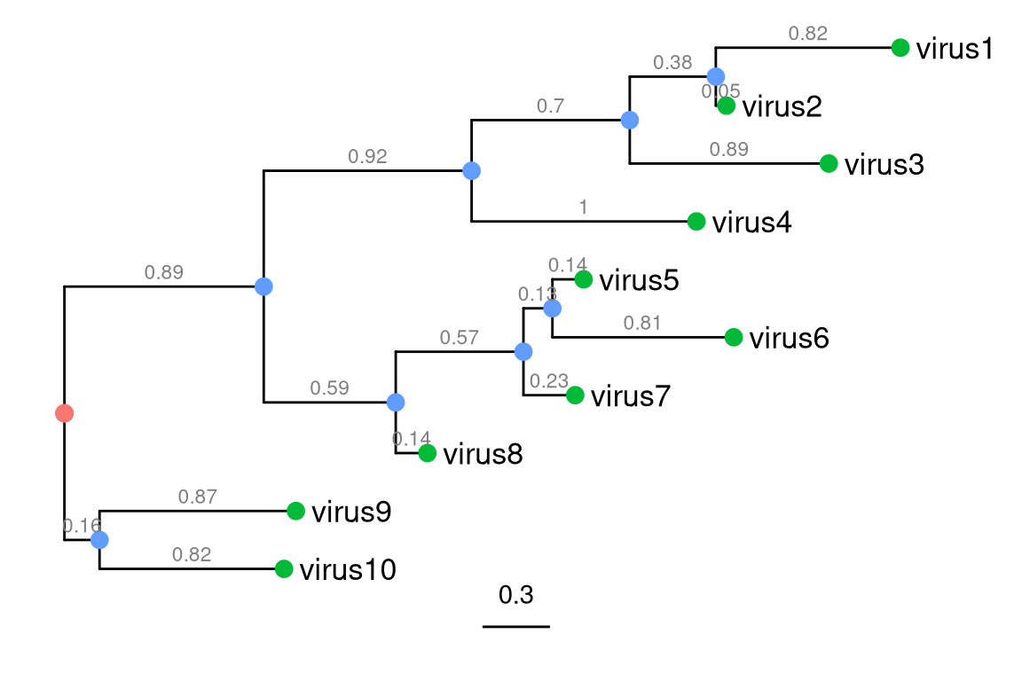
Figure 1.1: Components of a phylogenetic tree. External nodes (green circles), also called ‘tips’, represent actual organisms sampled and sequenced (e.g., virus in infectious disease research). They are the ‘taxa’ in the terminology of evolutionary biology. The internal nodes (blue circles) represent hypothetical ancestors for the tips. The root (red circle) is the common ancestor of all species in the tree. The horizontal lines are branches and represent evolutionary changes (grey number) measured in unit of time or genetic divergence. The bar at the bottom provides the scale of these branch lengths.
Phylogenetic tree can be constructed from genetic sequences using distance-based methods or character-based methods. Distance-based methods, including unweighted pair group method with arithmetic means (UPGMA) and Neighbor-joining (NJ), are based on the matrix of pairwise genetic distances calculated between sequences. The character-based methods, including maximum parsimony (MP) (Fitch 1971), maximum likelihood (ML) (Felsenstein 1981), and Bayesian Markov Chain Monte Carlo (BMCMC) method (Rannala and Yang 1996), are based on mathematical model that describes the evolution of genetic characters and search for the best phylogenetic tree according to their own optimality criteria.
Maximum Parsimony (MP) method assumes that the evolutionary change is rare and minimizes the amount of character-state changes (e.g., number of DNA substitutions). The criterion is similar to Occam’s razor, that the simplest hypothesis that can explains the data is the best hypothesis. Unweighted parsimony assumes mutations across different characters (nucleotides or amino acids) are equally likely while weighted method assume unequal likely of mutations (e.g., the third codon position is more liable than other codon positions; and the transition mutations have higher frequency than transversion). The concept of MP method is straightforward and intuitive, which is a probable reason for its popularity amongst biologists who care more about the research question rather than the computational details of the analysis. However, this method has a number of disadvantages, which in particular the tree inference can be biased by the well-known systematic error called long-branch attraction (LBA) that incorrectly infer distantly related lineages as closely related (Felsenstein 1978). This is because MP method poorly takes into consideration of many sequence evolution factors (e.g., reversals and convergence) that are hardly observable from the existing genetic data.
Maximum likelihood (ML) method and Bayesian Markov Chain Monte Carlo (BMCMC) method are the two most commonly used methods in phylogenetic tree construction and are most often used in scientific publications. ML and BMCMC methods require a substitution model of sequence evolution. Different sequence data have different substitution models to formulate the evolutionary process of DNA, codon and amino acid. There are several models for nucleotide substitution, including JC69, K2P, F81, HKY and GTR (Arenas 2015). These models can be used in conjunction with the rate variation across sites (denoted as +\(\Gamma\))) (Yang 1994) and the proportion of invariable sites (denoted as +I) (Shoemaker and Fitch 1989). Previous research (Lemmon and Moriarty 2004) had suggested that misspecification of substitution model might bias phylogenetic inference. Procedural testing for the best-fit substitution model is recommended.
The optimal criterion of ML method is to find the tree that maximizes the likelihood given the sequence data. The procedure of ML method is simple: calculating the likelihood of a tree and optimizing its topology and branches (and the substitution model parameters, if not fixed) until the best tree is found. Heuristic search such as those implemented in PhyML and RAxML, is often used to find the best tree based on the likelihood criterion. Bayesian method finds the tree that maximizes posterior probability by sampling trees through MCMC based on the given substitution model. One of the advantage of BMCMC is that parameter variance and tree topological uncertainty, included by the posterior clade probability, can be naturally and conveniently obtained from the sampling trees in MCMC process. Moreover, influence of topological uncertainty to other parameter estimates are also naturally integrated in the BMCMC phylogenetic framework.
In a simple phylogenetic tree, data associated with the tree branches/nodes could be the branch lengths (indicating genetic or time divergence) and lineage supports such as bootstrap values estimated from bootstrapping procedure or posterior clade probability summarized from the sampled trees in the BMCMC analysis.
1.2 Phylogenetic Tree Formats
There are several file formats designed to store phylogenetic trees and the data associated with the nodes and branches. The three commonly used formats are Newick1, NEXUS (Maddison et al. 1997) and Phylip (Felsenstein 1989). Some formats (e.g., NHX) are extended from Newick format. Newick and NEXUS formats are supported as input by most of the software in evolutionary biology, while some of the software tools output newer standard files (e.g., BEAST and MrBayes) by introducing new rules/data blocks for storing evolutionary inferences. On the other cases (e.g., PAML and r8s), output log files are only recognized by their own single software.
1.2.1 Newick tree format
The Newick tree format is the standard for representing trees in computer-readable form.
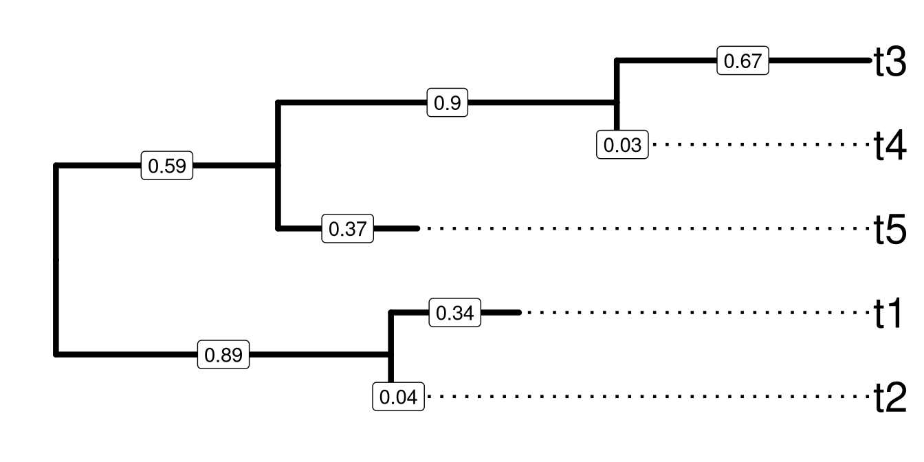
Figure 1.2: A sample tree for demonstrating Newick text to encode tree structure. Tips were aligned to right hand side and branch lengths were labelled on the middle of each branch.
The rooted tree shown in Figure 1.2 can be represented by the following sequence of characters as a newick tree text.
((t2:0.04,t1:0.34):0.89,(t5:0.37,(t4:0.03,t3:0.67):0.9):0.59); The tree text ends with semicolon. Internal nodes are represented by a pair of matched parentheses. Between the parentheses are descendant nodes of that node. For instance (t4:0.59, t1:0.37) represents the parent node of t4 and t1 that are the immediate descendants. Sibling nodes are separated by comma and tips are represented by their names. A branch length (from parent node to child node) is represented by a real number after the child node and preceded by a colon. Singular data (e.g., bootstrap values) associated with internal nodes or branches maybe encoded as node label and represented by the simple text/numbers before the colon.
Newick tree format was developed by Meacham in 1984 for the PHYLIP (Retief 2000) package. Newick format is now the most widely used tree format and used by PHYLIP, PAUP* (Wilgenbusch and Swofford 2003), TREE-PUZZLE (Schmidt et al. 2002), MrBayes and many other applications. Phylip tree format contains Phylip multiple sequence alignment (MSA) with a corresponding Newick tree text that was built based on the MSA sequences in the same file.
1.2.2 NEXUS tree format
The NEXUS format (Maddison et al. 1997) incorporates Newick tree text with related information organized into separated units known as blocks. A NEXUS block has the following structure:
#NEXUS
...
BEGIN characters;
...
END;
For example, the above example tree can be saved as a following NEXUS format:
#NEXUS
[R-package APE, Wed Nov  9 11:46:32 2016]

BEGIN TAXA;
	DIMENSIONS NTAX = 5;
	TAXLABELS
		t5
		t4
		t1
		t2
		t3
	;
END;
BEGIN TREES;
	TRANSLATE
		1	t5,
		2	t4,
		3	t1,
		4	t2,
		5	t3
	;
	TREE * UNTITLED = [&R] (1:0.89,((2:0.59,3:0.37):0.34,
	(4:0.03,5:0.67):0.9):0.04);
END;
Comments can be placed by using square brackets. Some blocks can be recognized by most of the programs including TAXA (contains information of taxa), DATA (contains data matrix, e.g., sequence alignment) and TREE (contains phylogenetic tree, i.e., Newick tree text). Notably, blocks can be very diversed and some of them are only be recognized by one particular program. For example NEXUS file exported by PAUP* has a paup block which contains PAUP* commands, whereas FigTree exports NEXUS file with a figtree block that contains visualization settings. NEXUS organizes different types of data into different blocks, whereas programs that support reading NEXUS can parse some blocks they recognized and ignore those they could not. This is a good mechanism to allow different programs to use the same format without crashing when unsupported types of data are present. Notably most of the programs only support parsing TAXA, DATA and TREE blocks, therefore a program/platform that could generically read all kinds of data blocks from the NEXUS would be useful for phylogenetic data integration.
The DATA block is widely used to store sequence alignment. For this purpose, user can store tree and sequence data in Phylip format which are essentially Phylip multiple sequence alignment and Newick tree text respectively. It is used in Phylogeny Inference Package (PHYLIP).
1.2.3 New Hampshire eXtended format
Newick, NEXUS and phylip are mainly designed to store phylogenetic tree and basic singular data associated with internal nodes or branches. In addition to the singular data annotation at branches and nodes (mentioned above), New Hampshire eXtended format (NHX), which is based on Newick (also called New Hampshire), was developed to introduce tags to associate multiple data fields with the tree nodes (both internal nodes and tips). Tags are placed after branch length and must be wrapped between [&&NHX and ] which makes it possible to compatible with NEXUS format as it defined characters between [ and ] as comments. NHX is also the output format of PHYLDOG (Boussau et al. 2013) and RevBayes (Höhna et al. 2016). A Tree Viewer (ATV) (Zmasek and Eddy 2001) is a java tool that supports displaying annotation data stored in NHX format, but this package is no more maintained.
Here is a sample tree from NHX definition document2:
(((ADH2:0.1[&&NHX:S=human],
ADH1:0.11[&&NHX:S=human]):0.05[&&NHX:S=primates:D=Y:B=100],ADHY:0.1[&&NHX:S=nematode],ADHX:0.12[&&NHX:S=insect]):0.1[&&NHX:S=metazoa:D=N],
(ADH4:0.09[&&NHX:S=yeast],ADH3:0.13[&&NHX:S=yeast],
ADH2:0.12[&&NHX:S=yeast],ADH1:0.11[&&NHX:S=yeast]):0.1[&&NHX:S=Fungi])
[&&NHX:D=N];
1.2.4 Jplace format
In order to store the NGS short reads mapped onto a phylogenetic tree (for the purpose of metagenomic classification), Matsen proposed jplace format for such phylogenetic placements (Matsen et al. 2012). Jplace format is based on JSON and contains four keys: tree, fields, placements, metadata and version. The tree value contains tree text extended from Newick tree format by putting the edge label in brackets (if available) after branch length and putting the edge number in curly braces after edge label. The fields value contains header information of placement data. The value of placements is a list of pqueries. Each pquery contains two keys: p for placements and n for name or nm for names with multiplicity. The value of p is a list of placement for that pqueries.
Here is a jplace sample file:
{
	"tree": "(((((((A:4{1},B:4{2}):6{3},C:5{4}):8{5},D:6{6}):
	3{7},E:21{8}):10{9},((F:4{10},G:12{11}):14{12},H:8{13}):
	13{14}):13{15},((I:5{16},J:2{17}):30{18},(K:11{19},
	L:11{20}):2{21}):17{22}):4{23},M:56{24});",
	"placements": [
	{"p":[24, -61371.300778, 0.333344, 0.000003, 0.003887],
	 "n":["AA"]
	},
	{"p":[[1, -61312.210786, 0.333335, 0.000001, 0.000003],
	      [2, -61322.210823, 0.333322, 0.000003, 0.000003],
	      [3, -61352.210823, 0.333322, 0.000961, 0.000003]],
	 "n":["BB"]
	},
	{"p":[[8, -61312.229128, 0.200011, 0.000001, 0.000003],
	      [9, -61322.229179, 0.200000, 0.000003, 0.000003],
	      [10, -61342.229223, 0.199992, 0.000003, 0.000003]],
	"n":["CC"]
	}
	],
	"metadata": {"info": "a jplace sample file"},
	"version" : 2,
	"fields": ["edge_num", "likelihood", "like_weight_ratio",
	"distal_length", "pendant_length"
	]
}
Jplace is the output format of pplacer (Frederick A. Matsen, Kodner, and Armbrust 2010) and Evolutionary Placement Algorithm (EPA) (Berger, Krompass, and Stamatakis 2011a). But these two programs do not contain tools to visualize placement results. Pplacer provides placeviz to convert jplace file to phyloXML or Newick formats which can be visualized by Archaeopteryx3.
1.2.5 Software outputs
RAxML (Stamatakis 2014) can output Newick format by storing the bootstrap values as internal node labels. Another way that RAxML supported is to place bootstrap value inside square brackets and after branch length. This could not be supported by most of the software that support Newick format where square brackets will be ignored.
BEAST (Bouckaert et al. 2014) output is based on NEXUS and it also introduce square brackets in the tree block to store evolutionary evidences inferred by BEAST. Inside brackets, curly braces may also incorporated if feature values have length more than 1 (e.g., HPD or range of substitution rate). These brackets are placed between node and branch length (i.e., after label if exists and before colon). Bracket is not defined in Newick format and is reserve character for NEXUS comment. So these information will be ignored for standard NEXUS parsers.
Here is a sample TREE block of the BEAST output:
tree TREE1 = [&R]
(((11[&length=9.4]:9.38,14[&length=6.4]:6.385096430786298)
[&length=25.7]:25.43,4[&length=9.1]:8.821663252749829)
[&length=3.0]:3.10,(12[&length=0.6]:0.56,
(10[&length=1.6]:1.56,(7[&length=5.2]:5.19,
((((2[&length=3.3]:3.26,(1[&length=1.3]:1.32,
(6[&length=0.8]:0.83,13[&length=0.8]:0.8311577761397366)
[&length=2.4]:2.48917886025146)
[&length=0.9]:0.9416178372674331)
[&length=0.4]:0.49,9[&length=1.7]:1.757288031101215)
[&length=2.4]:2.35,8[&length=2.1]:2.1125745387283246)
[&length=0.2]:0.23,(3[&length=3.3]:3.31,
(15[&length=5.2]:5.27,5[&length=3.2]:3.2710481368304585)
[&length=1.0]:1.0409443024626412)
[&length=1.9]:2.0372962536780435)
[&length=2.8]:2.8446835614595685)
[&length=5.3]:5.367459711197171)
[&length=2.0]:2.0037467863383043)
[&length=4.3]:4.360909907798238)[&length=0.0];
BEAST output can contain many different evolutionary inferences, depending of the analysis models defined in BEAUTi for running. For example in molecular clock analysis, it contains rate, length, height, posterior and corresponding HPD and range for uncertainty estimation. Rate is the estimated evolutionary rate of the branch. Length is the length of the branch in years. Height is the time from node to root while posterior is the Bayesian clade credibility value. The above example is the output tree of clock analysis and should contains these inferences. To save space, only the length estimation was shown above. Besides, MEGA (Kumar, Stecher, and Tamura 2016) also supports exporting tree in BEAST compatible Nexus format (see session 1.3.2).
MrBayes (Huelsenbeck and Ronquist 2001) is a program that uses Markov Chain Monte Carlo method to sample from the posterior probability distributions. Its output file annotates nodes and branches separately by two sets of square brackets. For example below, posterior clade probabilities for the node and branch length estimates for the branch:
tree con_all_compat = [&U]
(8[&prob=1.0]:2.94e-1[&length_mean=2.9e-1],10[&prob=1.0]:2.25e-1[&length_mean=2.2e-1],
((((1[&prob=1.0]:1.43e-1[&length_mean=1.4e-1],2[&prob=1.0]:1.92e-1[&length_mean=1.9e-1])
[&prob=1.0]:1.24e-1[&length_mean=1.2e-1],9[&prob=1.0]:2.27e-1[&length_mean=2.2e-1])
[&prob=1.0]:1.72e-1[&length_mean=1.7e-1],12[&prob=1.0]:5.11e-1[&length_mean=5.1e-1])
[&prob=1.0]:1.76e-1[&length_mean=1.7e-1],
(((3[&prob=1.0]:5.46e-2[&length_mean=5.4e-2],
(6[&prob=1.0]:1.03e-2[&length_mean=1.0e-2],7[&prob=1.0]:7.13e-3[&length_mean=7.2e-3])
[&prob=1.0]:6.93e-2[&length_mean=6.9e-2])
[&prob=1.0]:6.03e-2[&length_mean=6.0e-2],
(4[&prob=1.0]:6.27e-2[&length_mean=6.2e-2],5[&prob=1.0]:6.31e-2[&length_mean=6.3e-2])
[&prob=1.0]:6.07e-2[&length_mean=6.0e-2])
[&prob=1.0]:1.80e-1[&length_mean=1.8e-1],11[&prob=1.0]:2.37e-1[&length_mean=2.3e-1])
[&prob=1.0]:4.05e-1[&length_mean=4.0e-1])
[&prob=1.0]:1.16e+000[&length_mean=1.162699558201079e+000])
[&prob=1.0][&length_mean=0];
To save space, most of the inferences were removed and only contains prob for clade probability and length_mean for mean value of branch length. The full version of this file also contains prob_stddev, prob_range, prob(percent), prob+-sd for probability inferences and length_median, length_95%_HPD for every branch.
The BEAST and MrBayes outputs are expected to be parsed without inferences (dropped as comments) by software that support NEXUS. FigTree supports parsing BEAST and MrBayes outputs with inferences that can be used to display or annotate on the tree. But from there extracting these data for further analysis is still challenging.
HyPhy (Pond, Frost, and Muse 2005) could do a number of phylogenetic analysis, including ancestral sequence reconstruction. For ancestral sequence reconstruction, these sequences and the Newick tree text are stored in NEXUS format as the major analysis output. It did not completely follow the NEXUS definition and only put the ancestral node labels in TAXA instead of external node label. The MATRIX block contains sequence alignment of ancestral nodes which cannot be referred back to the tree stored in TREES block since it does not contains node labels. Here is the sample output (to save space, only the first 72bp of alignment are shown):
#NEXUS

[
Generated by HYPHY 2.0020110620beta(MP) for MacOS(Universal Binary)
	on Tue Dec 23 13:52:34 2014

]

BEGIN TAXA;
	DIMENSIONS NTAX = 13;
	TAXLABELS
		'Node1' 'Node2' 'Node3' 'Node4' 'Node5' 'Node12' 'Node13' 'Node15'
			'Node18' 'Node20' 'Node22' 'Node24' 'Node26' ;
END;

BEGIN CHARACTERS;
	DIMENSIONS NCHAR = 2148;
	FORMAT
		DATATYPE = DNA

		GAP=-
		MISSING=?
		NOLABELS
	;

MATRIX
 ATGGAAGACTTTGTGCGACAATGCTTCAATCCAATGATCGTCGAGCTTGCGGAAAAGGCAATGAAAGAATAT
 ATGGAAGACTTTGTGCGACAATGCTTCAATCCAATGATCGTCGAGCTTGCGGAAAAGGCAATGAAAGAATAT
 ATGGAAGACTTTGTGCGACAATGCTTCAATCCAATGATCGTCGAGCTTGCGGAAAAGGCAATGAAAGAATAT
 ATGGAAGACTTTGTGCGACAATGCTTCAATCCAATGATCGTCGAGCTTGCGGAAAAGGCAATGAAAGAATAT
 ATGGAAGACTTTGTGCGACAATGCTTCAATCCAATGATTGTCGAGCTTGCGGAAAAGGCAATGAAAGAATAT
 ATGGAAGACTTTGTGCGACAATGCTTCAATCCAATGATCGTCGAGCTTGCGGAAAAGGCAATGAAAGAATAT
 ATGGAAGACTTTGTGCGACAATGCTTCAATCCAATGATCGTCGAGCTTGCGGAAAAGGCAATGAAAGAATAT
 ATGGAAGACTTTGTGCGACAATGCTTCAATCCAATGATCGTCGAGCTTGCGGAAAAGGCAATGAAAGAATAT
 ATGGAAGACTTTGTGCGACAATGCTTCAATCCAATGATCGTCGAGCTTGCGGAAAAGGCAATGAAAGAATAT
 ATGGAAGACTTTGTGCGACAATGCTTCAATCCAATGATCGTCGAGCTTGCGGAAAAGGCAATGAAAGAATAT
 ATGGAAGACTTTGTGCGACAATGCTTCAATCCAATGATCGTCGAGCTTGCGGAAAAGGCAATGAAAGAATAT
 ATGGAAGACTTTGTGCGACAATGCTTCAATCCAATGATCGTCGAGCTTGCGGAAAAGGCAATGAAAGAATAT
 ATGGAAGACTTTGTGCGACAGTGCTTCAATCCAATGATCGTCGAGCTTGCGGAAAAGGCAATGAAAGAATAT
END;

BEGIN TREES;
	TREE tree = (K,N,(D,(L,(J,(G,((C,(E,O)),(H,(I,(B,(A,(F,M)))))))))));
END;
There are other applications that output rich information text that also contains phylogenetic trees with associated data. For example r8s (Sanderson 2003) output three trees in its log file, namely TREE, RATE and PHYLO for branches scaled by time, substitution rate, and absolute substitutions respectively.
Phylogenetic Analysis by Maximum Likelihood (PAML) (Yang 2007) is a package of programs for phylogenetic analyses of DNA or protein sequences. Two main programs, BaseML and CodeML, implement a variety of models. BaseML estimates tree topology, branch lengths and substitution parameters using a number of nucleotide substitution models available, including JC69, K80, F81, F84, HKY85, T92, TN93 and GTR. CodeML estimates synonymous and non-synonymous substitution rates, likelihood ratio test of positive selection under codon substitution models (Goldman and Yang 1994).
BaseML outputs mlb file that contains input sequence (taxa) alignment and phylogenetic tree with branch length as well as substitution model and other parameters estimated. The supplementary result file, rst, contains sequence alignment (with ancestral sequence if perform reconstruction of ancestral sequences) and Naive Empirical Bayes (NBE) probabilities that each site in the alignment evolved. CodeML outputs mlc file that contains tree structure and estimation of synonymous and non-synonymous substitution rates. CodeML also output supplementary result file, rst, that is similar to BaseML except that site is defined as codon instead of nucleotide. Parsing these files can be tedious and would oftentimes need a number of post-processing steps and require expertise in programming (e.g. with Python4 or Perl5).
Introducing square brackets is quite common for storing extra information, including RAxML to store bootstrap value, NHX format for annotation, jplace for edge label and BEAST for evolutionary estimation, etc.. But the positions to place square brackets are not consistent in different software and the contents employ different rules for storing associated data, these properties make it difficult to parse associated data. For most of the software, they will just ignore square brackets and only parse the tree structure if the file is compatible. Some of them contains invalid characters (e.g. curly braces in tree field of jplace format) and even the tree structure can’t be parsed by standard parsers.
It is difficult to extract useful phylogeny/taxon-related information from the different analysis outputs produced by various evolutionary inference software, for displaying on the same phylogenetic tree and for further analysis. FigTree supports BEAST output, but not for most of other software outputs that contains evolutionary inferences or associated data. For those output rich text files (e.g. r8s, PAML, etc.), the tree structure cannot be parsed by any tree viewing software and users need expertise to manually extract the phylogenetic tree and other useful result data from the output file. However, such manual operation is slow and error-prone.
It was not easy to retrieve phylogenetic trees with evolutionary data from different analysis outputs of commonly used software in the field. Some of them (e.g., PAML output and jplace file) without software or programming library to support parsing file, while others (e.g., BEAST and MrBayes output) can be parsed without evolutionary inferences as they are stored in square brackets that will be omitted as comment by most of the software. Although FigTree support visualizing evolutionary statistics inferred by BEAST and MrBayes, extracting these data for further analysis is not supported. Different software packages implement different algorithms for different analyses (e.g., PAML for dN/dS, HyPhy for ancestral sequences and BEAST for skyline analysis). Therefore, in encountering the genomic sequence data, there is a desire need to efficiently and flexibly integrate different analysis inference results for comprehensive understanding, comparison and further analysis. This motivated us to develop the programming library to parse the phylogenetic trees and data from various sources.
1.3 Getting Tree Data with treeio
Phylogenetic trees are commonly used to present evolutionary relationships of species. Information associated with taxon species/strains may be further analyzed in the context of the evolutionary history depicted by the phylogenetic tree. For example, host information of the influenza virus strains in the tree could be studied to understand host range of a virus linage. Moreover, such meta-data (e.g., isolation host, time, location, etc.) directly associated with taxon strains are also often subjected to further evolutionary or comparative phylogenetic models and analyses, to infer their dynamics associated with the evolutionary or transmission processes of the virus. All these meta-data or other phenotypic or experimental data are stored either as the annotation data associated with the nodes or branches, and are often produced in inconsistent format by different analysis programs.
Getting trees into R is still limited. Newick and Nexus can be imported by several packages, including ape, phylobase. NeXML format can be parsed by RNeXML. However, analysis results from widely used software packages in this field are not well supported. SIMMAP output can be parsed by phyext2 and phytools. Although PHYLOCH can import BEAST and MrBayes output, only internal node attributes were parsed and tip attributes were ignore6. Many other software outputs are mainly required programming expertise to import the tree with associated data. Linking external data, including experimental and clinical data, to phylogeny is another obstacle for evolution biologists.
To fill the gap that most of the tree formats or software outputs cannot be parsed within the same software/platform, an R package treeio (Wang et al. 2020) was developed for parsing various tree file formats and outputs from common evolutionary analysis software. The treeio package is developed with the R programming language (R Core Team 2016). Not only the tree structure can be parsed but also the associated data and evolutionary inferences, including NHX annotation, clock rate inferences (from BEAST or r8s (Sanderson 2003) programs), snynonymous and non-synonymous substitutions (from CodeML), and ancestral sequence construction (from HyPhy, BaseML or CodeML), etc.. Currently, treeio is able to read the following file formats: Newick, Nexus, New Hampshire eXtended format (NHX), jplace and Phylip as well as the data outputs from the following analysis programs: ASTRAL, BEAST, EPA, HyPhy, MEGA, MrBayes, PAML, PHYLDOG, pplacer, r8s, RAxML and RevBayes etc. This is made possible with the several parser functions developed in treeio (Table 1.1) (Wang et al. 2020).
| Parser function | Description |
|---|---|
| read.astral | parsing output of ASTRAL |
| read.beast | parsing output of BEAST |
| read.codeml | parsing output of CodeML (rst and mlc files) |
| read.codeml_mlc | parsing mlc file (output of CodeML) |
| read.fasta | parsing FASTA format sequence file |
| read.hyphy | parsing output of HYPHY |
| read.hyphy.seq | parsing ancestral sequences from HYPHY output |
| read.iqtree | parsing IQ-Tree newick string, with ability to parse SH-aLRT and UFBoot support values |
| read.jplace | parsing jplace file including output of EPA and pplacer |
| read.jtree | parsing jtree format |
| read.mega | parsing MEGA Nexus output |
| read.mega_tabular | parsing MEGA tabular output |
| read.mrbayes | parsing output of MrBayes |
| read.newick | parsing newick string, with ability to parse node label as support values |
| read.nexus | parsing standard NEXUS file (re-exported from ape) |
| read.nhx | parsing NHX file including output of PHYLDOG and RevBayes |
| read.paml_rst | parsing rst file (output of BaseML or CodeML) |
| read.phylip | parsing phylip file (phylip alignment + newick string) |
| read.phylip.seq | parsing multiple sequence alignment from phylip file |
| read.phylip.tree | parsing newick string from phylip file |
| read.phyloxml | parsing phyloXML file |
| read.r8s | parsing output of r8s |
| read.raxml | parsing output of RAxML |
| read.tree | parsing newick string (re-exported from ape) |
The treeio package defines base
classes and functions for phylogenetic tree input and output. It is an
infrastructure that enables evolutionary evidences that inferred by commonly
used software packages to be used in R. For instance, dN/dS values or
ancestral sequences inferred
by CODEML (Yang 2007),
clade support values (posterior) inferred
by BEAST (Bouckaert et al. 2014) and short read placement
by
EPA (Berger, Krompass, and Stamatakis 2011b)
and pplacer (Frederick A Matsen, Kodner, and Armbrust 2010). These
evolutionary evidences can be further analyzed in R and used to annotate
phylogenetic tree using ggtree
(Yu et al. 2017). The growth of analysis tools and models introduces
a challenge to integrate different varieties of data and analysis results from
different sources for an integral analysis on the the same phylogenetic tree
background. The treeio package (Wang et al. 2020)
provides a merge_tree function to allow combining tree data obtained from
different sources. In addition, treeio also enables external data to be linked to phylogenetic tree structure.
After parsing, storage of the tree structure with associated data is made
through a S4 class, treedata, defined in the tidytree package. These parsed data
are mapped to the tree branches and nodes inside treedata object, so that they
can be efficiently used to visually annotate the tree
using ggtree package (Yu et al. 2017) (described in Chapter 4 and 5).
A programmable platform for phylogenetic data parsing, integration and annotations as such makes us easier to identify the evolutionary dynamics and correlation patterns (Figure 1.3).
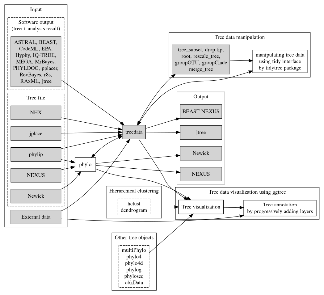
Figure 1.3: Overview of the treeio package and its relations with tidytree and ggtree. Treeio supports parsing a tree with data from a number of file formats and software outputs. A treedata object stores a phylogenetic tree with node/branch-associated data. Treeio provides several functions to manipulate a tree with data. Users can convert the treedata object into a tidy data frame (each row represents a node in the tree and each column represents a variable) and process the tree with data using the tidy interface implemented in tidytree. The tree can be extracted from the treedata object and exported to a Newick and NEXUS file or can be exported with associated data into a single file (either in the BEAST NEXUS or jtree format). Associated data stored in the treedata object can be used to annotate the tree using ggtree. In addition, ggtree supports a number of tree objects, including phyloseq for microbiome data and obkData for outbreak data. The phylo, multiPhylo (ape package), phylo4, phylo4d (phylobase package), phylog (ade4 package), phyloseq (phyloseq package), and obkData (OutbreakTools package) are tree objects defined by the R community to store tree with or without domain-specific data. All these tree objects as well as hierachical clustering results (e.g., hclust and dendrogram objects) are supported by ggtree.
1.3.1 Overview of treeio
The treeio package (Wang et al. 2020) defined S4 classes for storing phylogenetic tree with diverse types of associated data or covariates from different sources including analysis outputs from different software packages. It also defined corresponding parser functions for parsing phylogenetic tree with annotation data and stored as data object in R for further manipulation or analysis (see Table 1.1). Several accessor functions were defined to facilitate accessing the tree annotation data, including get.fields for obtaining annotation features available in the tree object, get.placements for obtaining the phylogenetic placement results (i.e., output of pplacer, EPA, etc.), get.subs for obtaining the genetic substitutions from parent node to child node, and get.tipseq for getting the tip sequences.
The S3 class, phylo, which was defined in ape (Paradis, Claude, and Strimmer 2004) package, is widely used in R community and many packages. As treeio uses S4 class, to enable those available R packages to analyze the tree imported by treeio, treeio provides as.phylo function to convert treeio-generated tree object to phylo object that only contains tree structure without annotation data. In the other way, treeio also provides as.treedata function to convert phylo object with evolutionary analysis result (e.g., bootstrap values calculated by ape or ancestral states inferred by phangorn (Schliep 2011) etc) to be stored as a treedata S4 object, making it easy to map the data to the tree structure and to be visualized using ggtree (Yu et al. 2017).
To allow integration of different kinds of data in phylogenetic tree, treeio (Wang et al. 2020) provides merge_tree function (details in section 2.2.1) for combining evolutionary statistics/evidences imported from different sources including those common tree files and outputs from analysis programs (Table 1.1). There are other information, such as sampling location, taxonomy information, experimental result and evolutionary traits, etc. that are stored in separate files with user-defined format. In treeio, we could read in these data from the users’ files using standard R IO functions, and attach them to the tree object by the full_join methods defined in tidytree and treeio packages (see also the %<+% operator defined in ggtree). After attaching, the data will become the attributes associated with nodes or branches, which can be compared with other data incorporated, or can be visually displayed on the tree.
To facilitate storing the merged data into a single file, treeio implemented write.baset and write.jtree function to export treedata object for storing complex data associated with the phylogenetic tree (see Chapter 3).
1.3.2 Function Demonstration
1.3.2.1 Parsing BEAST output
file <- system.file("extdata/BEAST", "beast_mcc.tree", package="treeio")
beast <- read.beast(file)
beast
## 'treedata' S4 object that stored information of
## '/home/ygc/R/library/treeio/extdata/BEAST/beast_mcc.tree'.
##
## ...@ phylo:
## Phylogenetic tree with 15 tips and 14 internal nodes.
##
## Tip labels:
## A_1995, B_1996, C_1995, D_1987, E_1996, F_1997, ...
##
## Rooted; includes branch lengths.
##
## with the following features available:
## 'height', 'height_0.95_HPD', 'height_median',
## 'height_range', 'length', 'length_0.95_HPD',
## 'length_median', 'length_range', 'posterior', 'rate',
## 'rate_0.95_HPD', 'rate_median', 'rate_range'.Since % is not a valid character in names, all the feature names that contain x% will convert to 0.x. For example, length_95%_HPD will be changed to length_0.95_HPD.
Not only tree structure but also all the features inferred by BEAST will be stored in the S4 object. These features can be used for tree annotation (Figure 5.7).
1.3.2.2 Parsing MEGA output
MEGA (Kumar, Stecher, and Tamura 2016) supports exporting trees in three distinct formats: Newick, tabular and Nexus. The Newick file can be parsed using the read.tree or read.newick functions. MEGA Nexus file is similar to BEAST Nexus and treeio (Wang et al. 2020) provides read.mega function to parse the tree.
file <- system.file("extdata/MEGA7", "mtCDNA_timetree.nex", package = "treeio")
read.mega(file)
## 'treedata' S4 object that stored information of
## '/home/ygc/R/library/treeio/extdata/MEGA7/mtCDNA_timetree.nex'.
##
## ...@ phylo:
## Phylogenetic tree with 7 tips and 6 internal nodes.
##
## Tip labels:
## homo_sapiens, chimpanzee, bonobo, gorilla, orangutan, sumatran, ...
##
## Rooted; includes branch lengths.
##
## with the following features available:
## 'branch_length', 'data_coverage', 'rate', 'reltime',
## 'reltime_0.95_CI', 'reltime_stderr'.The tabular output contains tree and associated information (divergence time in this example) in a tabular flat text file. The read.mega_tabular function can parse the tree with data simultaneously.
file <- system.file("extdata/MEGA7", "mtCDNA_timetree_tabular.txt", package = "treeio")
read.mega_tabular(file)
## 'treedata' S4 object that stored information of
## '/home/ygc/R/library/treeio/extdata/MEGA7/mtCDNA_timetree_tabular.txt'.
##
## ...@ phylo:
## Phylogenetic tree with 7 tips and 6 internal nodes.
##
## Tip labels:
## chimpanzee, bonobo, homo sapiens, gorilla, orangutan, sumatran, ...
## Node labels:
## [1] "" "" "demoLabel2" ""
## [5] "" ""
##
## Rooted; no branch lengths.
##
## with the following features available:
## 'RelTime', 'CI_Lower', 'CI_Upper', 'Rate',
## 'Data Coverage'.1.3.2.3 Parsing MrBayes output
file <- system.file("extdata/MrBayes", "Gq_nxs.tre", package="treeio")
read.mrbayes(file)
## 'treedata' S4 object that stored information of
## '/home/ygc/R/library/treeio/extdata/MrBayes/Gq_nxs.tre'.
##
## ...@ phylo:
## Phylogenetic tree with 12 tips and 10 internal nodes.
##
## Tip labels:
## B_h, B_s, G_d, G_k, G_q, G_s, ...
##
## Unrooted; includes branch lengths.
##
## with the following features available:
## 'length_0.95HPD', 'length_mean', 'length_median', 'prob',
## 'prob_range', 'prob_stddev', 'prob_percent', 'prob+-sd'.1.3.2.4 Parsing PAML output
The read.paml_rst function can parse rst file
from BASEML
and CODEML. The only
difference is the space in the sequences.
For BASEML, each ten bases
are separated by one space, while
for CODEML, each three bases
(triplet) are separated by one space.
brstfile <- system.file("extdata/PAML_Baseml", "rst", package="treeio")
brst <- read.paml_rst(brstfile)
brst
## 'treedata' S4 object that stored information of
## '/home/ygc/R/library/treeio/extdata/PAML_Baseml/rst'.
##
## ...@ phylo:
## Phylogenetic tree with 15 tips and 13 internal nodes.
##
## Tip labels:
## A, B, C, D, E, F, ...
## Node labels:
## 16, 17, 18, 19, 20, 21, ...
##
## Unrooted; includes branch lengths.
##
## with the following features available:
## 'subs', 'AA_subs'.Similarly, we can parse the rst file from CODEML.
crstfile <- system.file("extdata/PAML_Codeml", "rst", package="treeio")
## type can be one of "Marginal" or "Joint"
crst <- read.paml_rst(crstfile, type = "Joint")
crst
## 'treedata' S4 object that stored information of
## '/home/ygc/R/library/treeio/extdata/PAML_Codeml/rst'.
##
## ...@ phylo:
## Phylogenetic tree with 15 tips and 13 internal nodes.
##
## Tip labels:
## A, B, C, D, E, F, ...
## Node labels:
## 16, 17, 18, 19, 20, 21, ...
##
## Unrooted; includes branch lengths.
##
## with the following features available:
## 'subs', 'AA_subs'.Ancestral sequences inferred by BASEML or CODEML via marginal or joint ML reconstruction methods will be stored in the S4 object and mapped to tree nodes. treeio (Wang et al. 2020) will automatically determine the substitutions between the sequences at the both ends of each branch. Amino acid substitution will also be determined by translating nucleotide sequences to amino acid sequences. These computed substitutions will also be stored in the S4 object for efficient tree annotation later (Figure 5.9).
CODEML infers selection
pressure and estimated dN/dS, dN and dS. These information are
stored in output file mlc, which can be parsed by read.codeml_mlc function.
mlcfile <- system.file("extdata/PAML_Codeml", "mlc", package="treeio")
mlc <- read.codeml_mlc(mlcfile)
mlc
## 'treedata' S4 object that stored information of
## '/home/ygc/R/library/treeio/extdata/PAML_Codeml/mlc'.
##
## ...@ phylo:
## Phylogenetic tree with 15 tips and 13 internal nodes.
##
## Tip labels:
## A, B, C, D, E, F, ...
## Node labels:
## 16, 17, 18, 19, 20, 21, ...
##
## Unrooted; includes branch lengths.
##
## with the following features available:
## 't', 'N', 'S', 'dN_vs_dS', 'dN', 'dS', 'N_x_dN', 'S_x_dS'.In previous session, we separately parsed rst and mlc files. However, they
can also be parsed together using read.codeml function.
## tree can be one of "rst" or "mlc" to specify
## using tree from which file as base tree in the object
ml <- read.codeml(crstfile, mlcfile, tree = "mlc")
ml
## 'treedata' S4 object that stored information of
## '/home/ygc/R/library/treeio/extdata/PAML_Codeml/rst',
## '/home/ygc/R/library/treeio/extdata/PAML_Codeml/mlc'.
##
## ...@ phylo:
## Phylogenetic tree with 15 tips and 13 internal nodes.
##
## Tip labels:
## A, B, C, D, E, F, ...
## Node labels:
## 16, 17, 18, 19, 20, 21, ...
##
## Unrooted; includes branch lengths.
##
## with the following features available:
## 'subs', 'AA_subs', 't', 'N', 'S', 'dN_vs_dS', 'dN', 'dS',
## 'N_x_dN', 'S_x_dS'.All the features in both rst and mlc files were imported into a single S4 object and hence are available for further annotation and visualization. For example, we can annotate and display both dN/dS (from mlc file) and amino acid substitutions (derived from rst file) on the same phylogenetic tree (Yu et al. 2017).
1.3.2.5 Parsing HyPhy output
Ancestral sequences inferred by HyPhy are
stored in the Nexus output file, which contains the tree topology and ancestral
sequences. To parse this data file, users can use the read.hyphy.seq function.
ancseq <- system.file("extdata/HYPHY", "ancseq.nex", package="treeio")
read.hyphy.seq(ancseq)
## 13 DNA sequences in binary format stored in a list.
##
## All sequences of same length: 2148
##
## Labels:
## Node1
## Node2
## Node3
## Node4
## Node5
## Node12
## ...
##
## Base composition:
## a c g t
## 0.335 0.208 0.237 0.220
## (Total: 27.92 kb)To map the sequences on the tree, user should also provide an internal-node-labelled tree. If users want to determine substitution, they need also provide tip sequences.
nwk <- system.file("extdata/HYPHY", "labelledtree.tree", package="treeio")
tipfas <- system.file("extdata", "pa.fas", package="treeio")
hy <- read.hyphy(nwk, ancseq, tipfas)
hy
## 'treedata' S4 object that stored information of
## '/home/ygc/R/library/treeio/extdata/HYPHY/labelledtree.tree'.
##
## ...@ phylo:
## Phylogenetic tree with 15 tips and 13 internal nodes.
##
## Tip labels:
## K, N, D, L, J, G, ...
## Node labels:
## Node1, Node2, Node3, Node4, Node5, Node12, ...
##
## Unrooted; includes branch lengths.
##
## with the following features available:
## 'subs', 'AA_subs'.1.3.2.6 Parsing r8s output
r8s uses parametric, semiparametric and nonparametric methods to relax molecular clock to allow better estimations of divergence times and evolution rates (Sanderson 2003). It outputs three trees in log file, namely TREE, RATO and PHYLO for time tree, rate tree and absolute substitution tree respectively.
Time tree is scaled by divergence time, rate tree is scaled by substitution rate and absolute substitution tree is scaled by absolute number of substitution. After parsing the file, all these three trees are stored in a multiPhylo object (Figure 4.15).
r8s <- read.r8s(system.file("extdata/r8s", "H3_r8s_output.log", package="treeio"))
r8s
## 3 phylogenetic trees1.3.2.7 Parsing output of RAxML bootstraping analysis
RAxML bootstraping analysis
output a Newick tree text that is not standard as it stores bootstrap values
inside square brackets after branch lengths. This file usually cannot be parsed
by traditional Newick parser, such as ape::read.tree. The function
read.raxml can read such file and stored the bootstrap as an additional
features, which can be used to display on the tree or used to color tree
branches, etc..
raxml_file <- system.file("extdata/RAxML", "RAxML_bipartitionsBranchLabels.H3", package="treeio")
raxml <- read.raxml(raxml_file)
raxml
## 'treedata' S4 object that stored information of
## '/home/ygc/R/library/treeio/extdata/RAxML/RAxML_bipartitionsBranchLabels.H3'.
##
## ...@ phylo:
## Phylogenetic tree with 64 tips and 62 internal nodes.
##
## Tip labels:
## A_Hokkaido_M1_2014_H3N2_2014, A_Czech_Republic_1_2014_H3N2_2014, FJ532080_A_California_09_2008_H3N2_2008, EU199359_A_Pennsylvania_05_2007_H3N2_2007, EU857080_A_Hong_Kong_CUHK69904_2006_H3N2_2006, EU857082_A_Hong_Kong_CUHK7047_2005_H3N2_2005, ...
##
## Unrooted; includes branch lengths.
##
## with the following features available:
## 'bootstrap'.1.3.2.8 Parsing NHX tree
NHX (New Hampshire eXtended) format is an extension of Newick by introducing NHX tags. NHX is commonly used in phylogenetics software, including PHYLDOG (Boussau et al. 2013), RevBayes (Höhna et al. 2014), for storing statistical inferences. The following codes imported a NHX tree with associated data inferred by PHYLDOG (Figure 3.1A).
nhxfile <- system.file("extdata/NHX", "phyldog.nhx", package="treeio")
nhx <- read.nhx(nhxfile)
nhx
## 'treedata' S4 object that stored information of
## '/home/ygc/R/library/treeio/extdata/NHX/phyldog.nhx'.
##
## ...@ phylo:
## Phylogenetic tree with 16 tips and 15 internal nodes.
##
## Tip labels:
## Prayidae_D27SS7@2825365, Kephyes_ovata@2606431, Chuniphyes_multidentata@1277217, Apolemia_sp_@1353964, Bargmannia_amoena@263997, Bargmannia_elongata@946788, ...
##
## Rooted; includes branch lengths.
##
## with the following features available:
## 'Ev', 'S', 'ND'.1.3.2.9 Parsing Phylip tree
Phylip format contains multiple sequence alignment of taxa in Phylip sequence
format with corresponding Newick tree text that was built from taxon sequences.
Multiple sequence alignment can be sorted based on the tree structure and displayed at
the right hand side of the tree using ggtree (see also the msaplot function and Basic Protocol 5 of (Yu 2020)).
phyfile <- system.file("extdata", "sample.phy", package="treeio")
phylip <- read.phylip(phyfile)
phylip
## 'treedata' S4 object that stored information of
## '/home/ygc/R/library/treeio/extdata/sample.phy'.
##
## ...@ phylo:
## Phylogenetic tree with 15 tips and 13 internal nodes.
##
## Tip labels:
## K, N, D, L, J, G, ...
##
## Unrooted; no branch lengths.1.3.2.10 Parsing EPA and pplacer output
EPA
(Berger, Krompass, and Stamatakis 2011b) and PPLACER
(Frederick A Matsen, Kodner, and Armbrust 2010) have common output file format, jplace, which can be
parsed by read.jplace() function.
jpf <- system.file("extdata/EPA.jplace",  package="treeio")
jp <- read.jplace(jpf)
print(jp)
## 'treedata' S4 object that stored information of
## '/home/ygc/R/library/treeio/extdata/EPA.jplace'.
##
## ...@ phylo:
## Phylogenetic tree with 493 tips and 492 internal nodes.
##
## Tip labels:
## CIR000447A, CIR000479, CIR000078, CIR000083, CIR000070, CIR000060, ...
##
## Rooted; includes branch lengths.
##
## with the following features available:
## 'nplace'.The number of evolutionary placement on each branch will be calculated and stored as the nplace feature, which can be mapped to line size and/or color using ggtree (Yu et al. 2017).
1.3.2.11 Parsing jtree format
The jtree is a JSON based format that was defined in
this treeio package (Wang et al. 2020) to support tree
data inter change (see session 3.3).
Phylogenetic tree with associated data can be exported to a single jtree
file using write.jtree function. The jtree can be easily parsed using any
JSON parser. The jtree format contains three keys: tree, data and metadata.
The tree value contains tree text extended from Newick tree format by putting
the edge number in curly braces after branch length. The data value contains
node/branch-specific data, while metadata value contains additional meta information.
jtree_file <- tempfile(fileext = '.jtree')
write.jtree(beast, file = jtree_file)
read.jtree(file = jtree_file)
## 'treedata' S4 object that stored information of
## '/tmp/RtmpvGnYhp/file55a5554175e02.jtree'.
##
## ...@ phylo:
## Phylogenetic tree with 15 tips and 14 internal nodes.
##
## Tip labels:
## K_2013, N_2010, D_1987, L_1980, J_1983, G_1992, ...
##
## Rooted; includes branch lengths.
##
## with the following features available:
## 'height', 'height_0.95_HPD', 'height_range', 'length',
## 'length_0.95_HPD', 'length_median', 'length_range', 'rate',
## 'rate_0.95_HPD', 'rate_median', 'rate_range',
## 'height_median', 'posterior'.1.3.3 Converting other tree-like object to phylo or treedata object
To extend the application scopes of treeio, tidytree and ggtree, treeio (Wang et al. 2020) provides several as.phylo and as.treedata methods to convert other tree-like objects, such as phylo4d and pml, to phylo or treedata object. So that users can easily mapping associated data to the tree structure, exporting tree with/without data to a single file, manipulating and visualizing tree with/without data. These convert functions (Table 1.2) create the possibility of using tidytree to process tree using tidy interface and ggtree to visualize tree using grammar of graphic syntax.
| Convert function | Supported object | Description |
|---|---|---|
| as.phylo | ggtree | convert ggtree object to phylo object |
| igraph | convert igraph object (only tree graph supported) to phylo object | |
| phylo4 | convert phylo4 object to phylo object | |
| pvclust | convert pvclust object to phylo object | |
| treedata | convert treedata object to phylo object | |
| as.treedata | ggtree | convert ggtree object to treedata object |
| phylo4 | convert phylo4 object to treedata object | |
| phylo4d | convert phylo4d object to treedata object | |
| pml | convert pml object to treedata object | |
| pvclust | convert pvclust object to treedata object |
Here, we used pml object which was defined in the phangorn package, as an example. The pml() function computes the likelihood of a phylogenetic tree given a sequence alignment and a model and the optim.pml() function optimizes different model parameters. The output is a pml object and it can be converted to a treedata object using as.treedata provided by treeio (Wang et al. 2020). The amino acid substitution (ancestral sequence estimated by pml) that stored in the treedata object can be visualized using ggtree as demonstrated in Figure 1.4.
library(phangorn)
treefile <- system.file("extdata", "pa.nwk", package="treeio")
tre <- read.tree(treefile)
tipseqfile <- system.file("extdata", "pa.fas", package="treeio")
tipseq <- read.phyDat(tipseqfile,format="fasta")
fit <- pml(tre, tipseq, k=4)
fit <- optim.pml(fit, optNni=FALSE, optBf=T, optQ=T,
                 optInv=T, optGamma=T, optEdge=TRUE,
                 optRooted=FALSE, model = "GTR",
				 control = pml.control(trace =0))

pmltree <- as.treedata(fit)
ggtree(pmltree) + geom_text(aes(x=branch, label=AA_subs, vjust=-.5))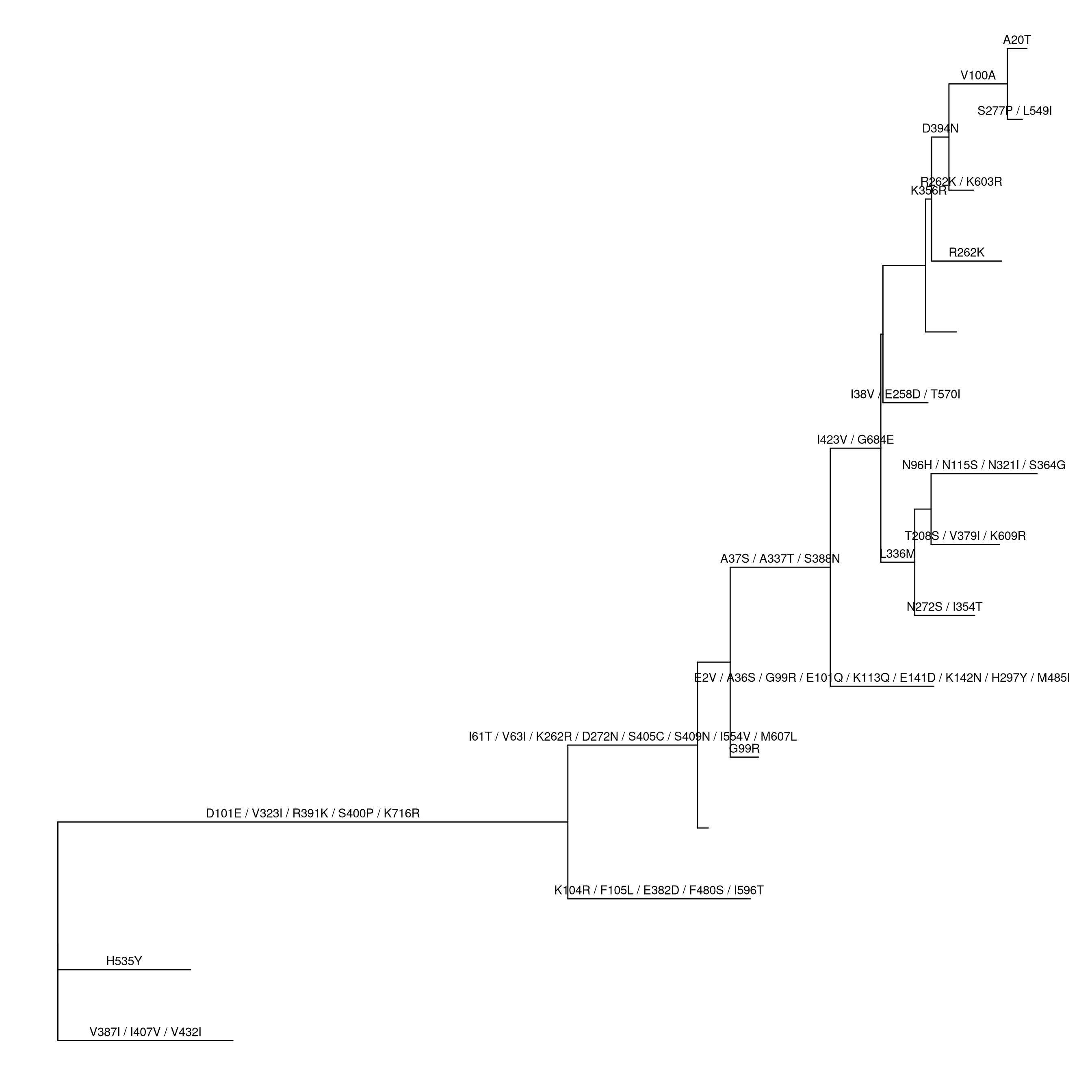
Figure 1.4: Converting pml object to treedata object.
1.3.4 Getting information from treedata object
After the tree was imported, users may want to extract information that stored
in the treedata object. treeio provides several accessor
methods to extract tree structure, features/attributes that stored in the object
and their corresponding values.
The get.tree or as.phylo methods can convert the treedata object to
phylo object which is the fundamental tree object in the R community and
many packages work with phylo object.
beast_file <- system.file("examples/MCC_FluA_H3.tree", package="ggtree")
beast_tree <- read.beast(beast_file)
# or get.tree
as.phylo(beast_tree)
##
## Phylogenetic tree with 76 tips and 75 internal nodes.
##
## Tip labels:
## A/Hokkaido/30-1-a/2013, A/New_York/334/2004, A/New_York/463/2005, A/New_York/452/1999, A/New_York/238/2005, A/New_York/523/1998, ...
##
## Rooted; includes branch lengths.The get.fields method return a vector of features/attributes that stored in
the object and associated with the phylogeny.
get.fields(beast_tree)## [1] "height" "height_0.95_HPD" "height_median"
## [4] "height_range" "length" "length_0.95_HPD"
## [7] "length_median" "length_range" "posterior"
## [10] "rate" "rate_0.95_HPD" "rate_median"
## [13] "rate_range"The get.data method return a tibble of all the associated data.
get.data(beast_tree)## # A tibble: 151 x 14
## height height_0.95_HPD height_median height_range length
## <dbl> <list> <dbl> <list> <dbl>
## 1 19 <dbl [2]> 19 <dbl [2]> 2.34
## 2 17 <dbl [2]> 17 <dbl [2]> 1.18
## 3 14 <dbl [2]> 14 <dbl [2]> 0.966
## 4 12 <dbl [2]> 12 <dbl [2]> 1.87
## 5 9 <dbl [2]> 9 <dbl [2]> 2.93
## 6 10 <dbl [2]> 10 <dbl [2]> 0.827
## 7 10 <dbl [2]> 10 <dbl [2]> 0.834
## 8 10.8 <dbl [2]> 10.8 <dbl [2]> 0.233
## 9 9 <dbl [2]> 9 <dbl [2]> 1.28
## 10 9 <dbl [2]> 9 <dbl [2]> 0.414
## # … with 141 more rows, and 9 more variables:
## # length_0.95_HPD <list>, length_median <dbl>,
## # length_range <list>, posterior <dbl>, rate <dbl>,
## # rate_0.95_HPD <list>, rate_median <dbl>,
## # rate_range <list>, node <int>If users are only interesting a subset of the features/attributes return by
get.fields, they can extract the information from the output of get.data or
directly subset the data by [ or [[.
beast_tree[, c("node", "height")]## # A tibble: 151 x 2
## node height
## <int> <dbl>
## 1 10 19
## 2 9 17
## 3 36 14
## 4 31 12
## 5 29 9
## 6 28 10
## 7 39 10
## 8 90 10.8
## 9 16 9
## 10 2 9
## # … with 141 more rowshead(beast_tree[["height_median"]])## height_median1 height_median2 height_median3 height_median4
## 19 17 14 12
## height_median5 height_median6
## 9 101.4 Summary
Software tools for inferring molecular evolution (e.g., ancestral states, molecular dating and selection pressure, etc.) are proliferating, but there is no single data format that is used by all different programs and capable to store different types of phylogenetic data. Most of the software packages have their own unique output formats and these formats are not compatible with each other. Parsing software outputs is challenging, which restricts the joint analysis using different tools. The treeio (Wang et al. 2020) provides a set of functions (Table 1.1) for parsing various types of phylogenetic data files and a set of converter (Table 1.2) to convert tree-like object to phylo or treedata object. These phylogenetic data can be integrated together that allows further exploration and comparison. To date, most software tools in the field of molecular evolution are isolated and often not fully compatible with each other’s input and output files. These software tools are designed to do their own analysis and the outputs are often not readable in other software. No tools have been designed to unify the inference data from different analysis programs. An efficient incorporation of data from different inference methods can enhance the comparison and understanding of the study target, which may help discover new systematic patterns and generate new hypothesis.
As phylogenetic trees are growing in its application to identify patterns in evolutionary context, more different disciplines are employing phylogenetic trees in their research. For example, spatial ecologists may map the geographical positions of the organisms to their phylogenetic trees to understand the biogeography of the species (Schön et al. 2015); disease epidemiologists may incorporate the pathogen sampling time and locations into the phylogenetic analysis to infer the disease transmission dynamics in spatiotemporal space (He et al. 2013); microbiologists may determine the pathogenicity of different pathogen strains and map them into their phylogenetic trees to identify the genetic determinants of the pathogenicity (Bosi et al. 2016); genomic scientists may use the phylogenetic trees to help taxonomically classify their metagenomic sequence data (Gupta and Sharma 2015). A robust tool such as treeio to import and map different types of data into the phylogenetic tree is important to facilitate these phylogenetics-related research, or a.k.a ‘phylodynamics’. Such tool could also help integrate different metadata (time, geography, genotype, epidemiological information) and analysis results (selective pressure, evolutionary rates) at the highest level and provide a comprehensive understanding of the study organisms. In the field of influenza research, there have been such attemps of studying phylodynamics of the influenza virus by mapping different meta-data and analysis results on the same phylogenetic tree and evolutionary time scale (Lam et al. 2015).
References
Arenas, Miguel. 2015. “Trends in Substitution Models of Molecular Evolution.” Frontiers in Genetics 6 (October). https://doi.org/10.3389/fgene.2015.00319.
Berger, Simon A., Denis Krompass, and Alexandros Stamatakis. 2011a. “Performance, Accuracy, and Web Server for Evolutionary Placement of Short Sequence Reads Under Maximum Likelihood.” Systematic Biology, March, syr010. https://doi.org/10.1093/sysbio/syr010.
Berger, Simon A., Denis Krompass, and Alexandros Stamatakis. 2011a. “Performance, Accuracy, and Web Server for Evolutionary Placement of Short Sequence Reads Under Maximum Likelihood.” Systematic Biology, March, syr010. https://doi.org/10.1093/sysbio/syr010.
2011b. “Performance, Accuracy, and Web Server for Evolutionary Placement of Short Sequence Reads Under Maximum Likelihood.” Systematic Biology 60 (3): 291–302. https://doi.org/10.1093/sysbio/syr010.Bosi, Emanuele, Jonathan M. Monk, Ramy K. Aziz, Marco Fondi, Victor Nizet, and Bernhard Ø. Palsson. 2016. “Comparative Genome-Scale Modelling of Staphylococcus Aureus Strains Identifies Strain-Specific Metabolic Capabilities Linked to Pathogenicity.” Proceedings of the National Academy of Sciences of the United States of America 113 (26): E3801–E3809. https://doi.org/10.1073/pnas.1523199113.
Bouckaert, Remco, Joseph Heled, Denise Kühnert, Tim Vaughan, Chieh-Hsi Wu, Dong Xie, Marc A. Suchard, Andrew Rambaut, and Alexei J. Drummond. 2014. “BEAST 2: A Software Platform for Bayesian Evolutionary Analysis.” PLoS Comput Biol 10 (4): e1003537. https://doi.org/10.1371/journal.pcbi.1003537.
Boussau, Bastien, Gergely J. Szöllősi, Laurent Duret, Manolo Gouy, Eric Tannier, and Vincent Daubin. 2013. “Genome-Scale Coestimation of Species and Gene Trees.” Genome Research 23 (2): 323–30. https://doi.org/10.1101/gr.141978.112.
Felsenstein, J. 1981. “Evolutionary Trees from DNA Sequences: A Maximum Likelihood Approach.” Journal of Molecular Evolution 17 (6): 368–76.
Felsenstein, Joseph. 1989. “PHYLIP - Phylogeny Inference Package (Version 3.2).” Cladistics 5: 164–66.
Felsenstein, Joseph. 1978. “Cases in Which Parsimony or Compatibility Methods Will Be Positively Misleading.” Systematic Biology 27 (4): 401–10. https://doi.org/10.1093/sysbio/27.4.401.
Fitch, Walter M. 1971. “Toward Defining the Course of Evolution: Minimum Change for a Specific Tree Topology.” Systematic Zoology 20 (4): 406–16. https://doi.org/10.2307/2412116.
Goldman, N., and Z. Yang. 1994. “A Codon-Based Model of Nucleotide Substitution for Protein-Coding DNA Sequences.” Molecular Biology and Evolution 11 (5): 725–36.
Gupta, Ankit, and Vineet K Sharma. 2015. “Using the Taxon-Specific Genes for the Taxonomic Classification of Bacterial Genomes.” BMC Genomics 16 (1). https://doi.org/10.1186/s12864-015-1542-0.
He, Ya-Qing, Long Chen, Wen-Bo Xu, Hong Yang, Han-Zhong Wang, Wen-Ping Zong, Hui-Xia Xian, et al. 2013. “Emergence, Circulation, and Spatiotemporal Phylogenetic Analysis of Coxsackievirus A6- and Coxsackievirus A10-Associated Hand, Foot, and Mouth Disease Infections from 2008 to 2012 in Shenzhen, China.” Journal of Clinical Microbiology 51 (11): 3560–6. https://doi.org/10.1128/JCM.01231-13.
Höhna, Sebastian, Tracy A. Heath, Bastien Boussau, Michael J. Landis, Fredrik Ronquist, and John P. Huelsenbeck. 2014. “Probabilistic Graphical Model Representation in Phylogenetics.” Systematic Biology 63 (5): 753–71. https://doi.org/10.1093/sysbio/syu039.
Höhna, Sebastian, Michael J. Landis, Tracy A. Heath, Bastien Boussau, Nicolas Lartillot, Brian R. Moore, John P. Huelsenbeck, and Fredrik Ronquist. 2016. “RevBayes: Bayesian Phylogenetic Inference Using Graphical Models and an Interactive Model-Specification Language.” Systematic Biology 65 (4): 726–36. https://doi.org/10.1093/sysbio/syw021.
Huelsenbeck, J. P., and F. Ronquist. 2001. “MRBAYES: Bayesian Inference of Phylogenetic Trees.” Bioinformatics (Oxford, England) 17 (8): 754–55.
Kumar, Sudhir, Glen Stecher, and Koichiro Tamura. 2016. “MEGA7: Molecular Evolutionary Genetics Analysis Version 7.0 for Bigger Datasets.” Molecular Biology and Evolution 33 (7): 1870–4. https://doi.org/10.1093/molbev/msw054.
Lam, Tommy Tsan-Yuk, Boping Zhou, Jia Wang, Yujuan Chai, Yongyi Shen, Xinchun Chen, Chi Ma, et al. 2015. “Dissemination, Divergence and Establishment of H7N9 Influenza Viruses in China.” Nature 522 (7554): 102–5. https://doi.org/10.1038/nature14348.
Lemmon, Alan R., and Emily C. Moriarty. 2004. “The Importance of Proper Model Assumption in Bayesian Phylogenetics.” Systematic Biology 53 (2): 265–77. https://doi.org/10.1080/10635150490423520.
Maddison, David R., David L. Swofford, Wayne P. Maddison, and David Cannatella. 1997. “Nexus: An Extensible File Format for Systematic Information.” Systematic Biology 46 (4): 590–621. https://doi.org/10.1093/sysbio/46.4.590.
Matsen, Frederick A., Noah G. Hoffman, Aaron Gallagher, and Alexandros Stamatakis. 2012. “A Format for Phylogenetic Placements.” PLoS ONE 7 (2): e31009. https://doi.org/10.1371/journal.pone.0031009.
Matsen, Frederick A., Robin B. Kodner, and E Virginia Armbrust. 2010. “Pplacer: Linear Time Maximum-Likelihood and Bayesian Phylogenetic Placement of Sequences onto a Fixed Reference Tree.” BMC Bioinformatics 11: 538. https://doi.org/10.1186/1471-2105-11-538.
Matsen, Frederick A, Robin B Kodner, and E Virginia Armbrust. 2010. “Pplacer: Linear Time Maximum-Likelihood and Bayesian Phylogenetic Placement of Sequences onto a Fixed Reference Tree.” BMC Bioinformatics 11 (1): 538. https://doi.org/10.1186/1471-2105-11-538.
Paradis, Emmanuel, Julien Claude, and Korbinian Strimmer. 2004. “APE: Analyses of Phylogenetics and Evolution in R Language.” Bioinformatics 20 (2): 289–90. https://doi.org/10.1093/bioinformatics/btg412.
Pond, Sergei L. Kosakovsky, Simon D. W. Frost, and Spencer V. Muse. 2005. “HyPhy: Hypothesis Testing Using Phylogenies.” Bioinformatics (Oxford, England) 21 (5): 676–79. https://doi.org/10.1093/bioinformatics/bti079.
Rannala, B., and Z. Yang. 1996. “Probability Distribution of Molecular Evolutionary Trees: A New Method of Phylogenetic Inference.” Journal of Molecular Evolution 43 (3): 304–11.
R Core Team. 2016. R: A Language and Environment for Statistical Computing. Vienna, Austria: R Foundation for Statistical Computing. https://www.R-project.org/.
Retief, J. D. 2000. “Phylogenetic Analysis Using PHYLIP.” Methods in Molecular Biology (Clifton, N.J.) 132: 243–58.
Sanderson, Michael J. 2003. “R8s: Inferring Absolute Rates of Molecular Evolution and Divergence Times in the Absence of a Molecular Clock.” Bioinformatics 19 (2): 301–2. https://doi.org/10.1093/bioinformatics/19.2.301.
Schliep, Klaus Peter. 2011. “Phangorn: Phylogenetic Analysis in R.” Bioinformatics 27 (4): 592–93. https://doi.org/10.1093/bioinformatics/btq706.
Schmidt, Heiko A., Korbinian Strimmer, Martin Vingron, and Arndt von Haeseler. 2002. “TREE-PUZZLE: Maximum Likelihood Phylogenetic Analysis Using Quartets and Parallel Computing.” Bioinformatics (Oxford, England) 18 (3): 502–4.
Schön, Isa, Rylan Shearn, Koen Martens, Annette Koenders, and Stuart Halse. 2015. “Age and Origin of Australian Bennelongia (Crustacea, Ostracoda).” Hydrobiologia 750 (1): 125–46. https://doi.org/10.1007/s10750-014-2159-z.
Shoemaker, J. S., and W. M. Fitch. 1989. “Evidence from Nuclear Sequences That Invariable Sites Should Be Considered When Sequence Divergence Is Calculated.” Molecular Biology and Evolution 6 (3): 270–89.
Stamatakis, Alexandros. 2014. “RAxML Version 8: A Tool for Phylogenetic Analysis and Post-Analysis of Large Phylogenies.” Bioinformatics, January, btu033. https://doi.org/10.1093/bioinformatics/btu033.
Wang, Li-Gen, Tommy Tsan-Yuk Lam, Shuangbin Xu, Zehan Dai, Lang Zhou, Tingze Feng, Pingfan Guo, et al. 2020. “Treeio: An R Package for Phylogenetic Tree Input and Output with Richly Annotated and Associated Data.” Molecular Biology and Evolution 37 (2): 599–603. https://doi.org/10.1093/molbev/msz240.
Wilgenbusch, James C., and David Swofford. 2003. “Inferring Evolutionary Trees with PAUP*.” Current Protocols in Bioinformatics Chapter 6 (February): Unit 6.4. https://doi.org/10.1002/0471250953.bi0604s00.
Yang, Z. 1994. “Maximum Likelihood Phylogenetic Estimation from DNA Sequences with Variable Rates over Sites: Approximate Methods.” Journal of Molecular Evolution 39 (3): 306–14.
Yang, Ziheng. 2007. “PAML 4: Phylogenetic Analysis by Maximum Likelihood.” Molecular Biology and Evolution 24 (8): 1586–91. https://doi.org/10.1093/molbev/msm088.
Yu, Guangchuang. 2020. “Using Ggtree to Visualize Data on Tree-Like Structures.” Current Protocols in Bioinformatics 69 (1): e96. https://doi.org/10.1002/cpbi.96.
Yu, Guangchuang, David K. Smith, Huachen Zhu, Yi Guan, and Tommy Tsan-Yuk Lam. 2017. “Ggtree: An R Package for Visualization and Annotation of Phylogenetic Trees with Their Covariates and Other Associated Data.” Methods in Ecology and Evolution 8 (1): 28–36. https://doi.org/10.1111/2041-210X.12628.
Zmasek, Christian M., and Sean R. Eddy. 2001. “ATV: Display and Manipulation of Annotated Phylogenetic Trees.” Bioinformatics 17 (4): 383–84. https://doi.org/10.1093/bioinformatics/17.4.383.