Chapter 9 ggtree for other tree-like objects

9.1 ggtree for phylogenetic tree objects

The treeio packages allows parsing evolutionary inferences from a number of software outputs and linking external data to the tree structure. It serves as an infrastructure to bring evolutionary data to the R community. The ggtree package works seamlessly with treeio to visualize tree associated data to annotate the tree. The ggtree package is general tool for tree visualization and annotation and it fits the ecosystem of R packages. Most of the S3/S4 tree objects defined by other R packages are also supported by ggtree, including phylo(session 4.2), multiPhylo (session 4.4), phylo4, phylo4d, phyloseq and obkData. With ggtree, we are able to generate more complex tree graph which is not possible or easy to do with other packages. For example, the visualization of the phyloseq object in Figure 9.4 is not supported by the phyloseq package. The ggtree package also extend the possibility of linking external data to these tree object (Yu et al. 2018).

9.1.1 The phylo4 and phylo4d objects

The phylo4 and phylo4d are defined in the phylobase package. The phylo4 object is a S4 version of phylo, while phylo4d extends phylo4 with a data frame that contains trait data. The phylobase package provides plot method, which internally calls the treePlot function, to display the tree with the data. However there are some restrictions of the plot method, it can only plot numeric values for tree-associated data as bubbles and cannot generate figure legend. Phylobase doesn’t implement visualization method to display categorical values. Using associated data as visual characteristics such as color, size and shape, is also not supported. Although it is possible to color the tree using associated data, it requires users to extract the data and map them to color vector manually follow by passing the color vector to the plot method. This is tedious and error-prone since the order of the color vector needs to be consistent with the edge list stored in the object.

The ggtree package supports phylo4d object and all the associated data stored in the phylo4d object can be used directly to annotate the tree (Fig. ).

library(phylobase)
data(geospiza_raw)
g1 <- as(geospiza_raw$tree, "phylo4")
g2 <- phylo4d(g1, geospiza_raw$data, missing.data="warn")

d1 <- data.frame(x = seq(0.93, 1.15, length.out = 5),
                lab = names(geospiza_raw$data))

ggtree(g2) + geom_tippoint(aes(size = wingL), x = d1$x[1], shape = 1) + 
    geom_tippoint(aes(size = tarsusL), x = d1$x[2], shape = 1) + 
    geom_tippoint(aes(size = culmenL), x = d1$x[3], shape = 1) + 
    geom_tippoint(aes(size = beakD),   x = d1$x[4], shape = 1) + 
    geom_tippoint(aes(size = gonysW),  x = d1$x[5], shape = 1) + 
    scale_size_continuous(range = c(3,12), name="") + 
    geom_text(aes(x = x, y = 0, label = lab), data = d1, angle = 90) +
    geom_tiplab(offset = .3) + xlim(0, 1.3) +
    theme(legend.position = c(.1, .75))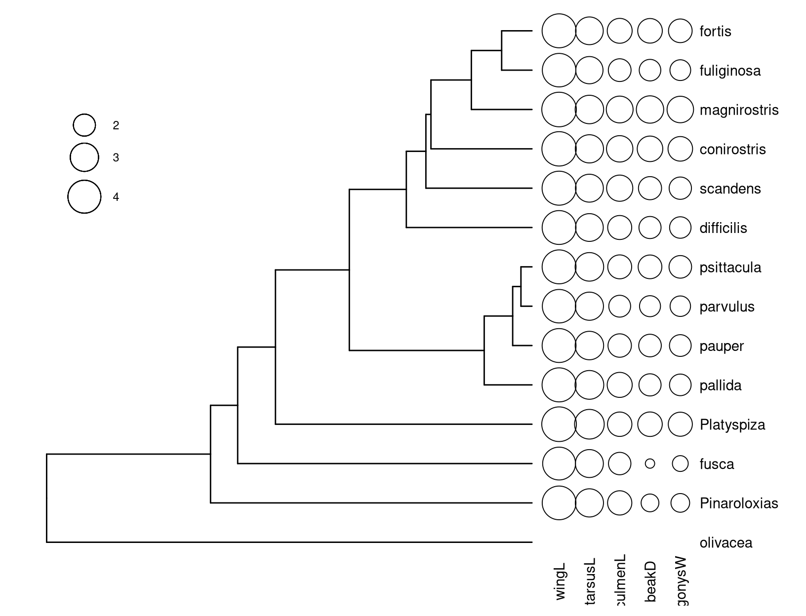

Figure 9.1: Visualizing phylo4d data using ggtree.

9.1.2 The phylog object

The phylog is defined in ade4 package. The package is designed for analyzing ecological data and provides newick2phylog, hclust2phylog and taxo2phylog functions to create phylogeny from Newick string, hierachical clustering result or a taxonomy. The phylog object is also supported by ggtree as demonstrated in Figure 9.2.

library(ade4)
data(taxo.eg)
tax <- as.taxo(taxo.eg[[1]])
print(tax)

##       genre famille ordre
## esp3     g1    fam1  ORD1
## esp1     g1    fam1  ORD1
## esp2     g1    fam1  ORD1
## esp4     g1    fam1  ORD1
## esp5     g1    fam1  ORD1
## esp6     g1    fam1  ORD1
## esp7     g1    fam1  ORD1
## esp8     g2    fam2  ORD2
## esp9     g3    fam2  ORD2
## esp10    g4    fam3  ORD2
## esp11    g5    fam3  ORD2
## esp12    g6    fam4  ORD2
## esp13    g7    fam4  ORD2
## esp14    g8    fam5  ORD2
## esp15    g8    fam5  ORD2

tax.phy <- taxo2phylog(as.taxo(taxo.eg[[1]]))
print(tax.phy)

## Phylogenetic tree with 15 leaves and 16 nodes
## $class: phylog
## $call: taxo2phylog(taxo = as.taxo(taxo.eg[[1]]))
## $tre: ((((esp3,esp1,esp2,esp4,e...15)l1g8)l2fam5)l3ORD2)Root; 
## 
##         class   length
## $leaves numeric 15    
## $nodes  numeric 16    
## $parts  list    16    
## $paths  list    31    
## $droot  numeric 31    
##         content                                     
## $leaves length of the first preceeding adjacent edge
## $nodes  length of the first preceeding adjacent edge
## $parts  subsets of descendant nodes                 
## $paths  path from root to node or leave             
## $droot  distance to root

ggtree(tax.phy) + geom_tiplab() + geom_nodelab(geom='label')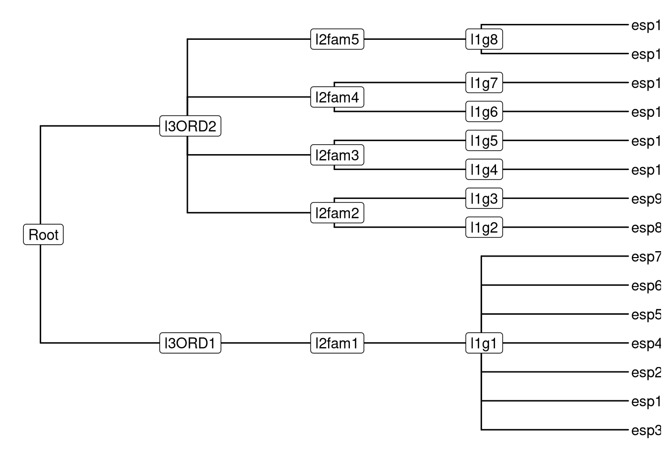

Figure 9.2: Visualizing phylog tree object.

9.1.3 The phyloseq object

The phyloseq class that defined in the phyloseq package was designed for storing microbiome data, including phylogenetic tree, associated sample data and taxonomy assignment. It can import data from popular pipelines, such as QIIME (Kuczynski et al. 2011), mothur (Schloss et al. 2009), DADA2 (Callahan et al. 2016) and PyroTagger (Kunin and Hugenholtz 2010), etc.. The ggtree supports visualizing the phylogenetic tree stored in phyloseq object and related data can be used to annotate the tree as demonstrated in Figure 9.3 and 9.4.

library(phyloseq)
library(scales)

data(GlobalPatterns)
GP <- prune_taxa(taxa_sums(GlobalPatterns) > 0, GlobalPatterns)
GP.chl <- subset_taxa(GP, Phylum=="Chlamydiae")

ggtree(GP.chl) + geom_text2(aes(subset=!isTip, label=label), hjust=-.2, size=4) +
  geom_tiplab(aes(label=Genus), hjust=-.3) +
  geom_point(aes(x=x+hjust, color=SampleType, shape=Family, size=Abundance),na.rm=TRUE) +
  scale_size_continuous(trans=log_trans(5)) +
  theme(legend.position="right")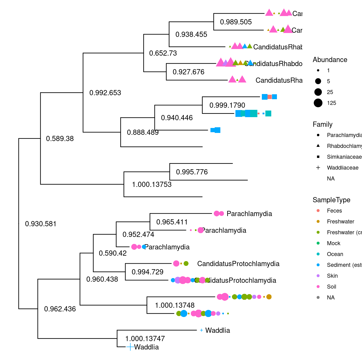

Figure 9.3: Visualizing phyloseq tree object.

Figure 9.3 reproduce output of phyloseq::plot_tree(). Users of phyloseq will find ggtree useful for visualizing microbiome data and for further annotation, since ggtree supports high-level of annotation using grammar of graphics and can add tree data layers that are not available in phyloseq.

library(ggridges)

data("GlobalPatterns")
GP <- GlobalPatterns
GP <- prune_taxa(taxa_sums(GP) > 600, GP)
sample_data(GP)$human <- get_variable(GP, "SampleType") %in% 
  c("Feces", "Skin") 

mergedGP <- merge_samples(GP, "SampleType")
mergedGP <- rarefy_even_depth(mergedGP,rngseed=394582)
mergedGP <- tax_glom(mergedGP,"Order") 

melt_simple <- psmelt(mergedGP) %>% 
  filter(Abundance < 120) %>% 
  select(OTU, val=Abundance)

ggtree(mergedGP) + 
  geom_tippoint(aes(color=Phylum), size=1.5) +
  geom_facet(mapping = aes(x=val,group=label, 
                           fill=Phylum),
            data = melt_simple, 
            geom = geom_density_ridges,
            panel="Abundance",  
            color='grey80', lwd=.3)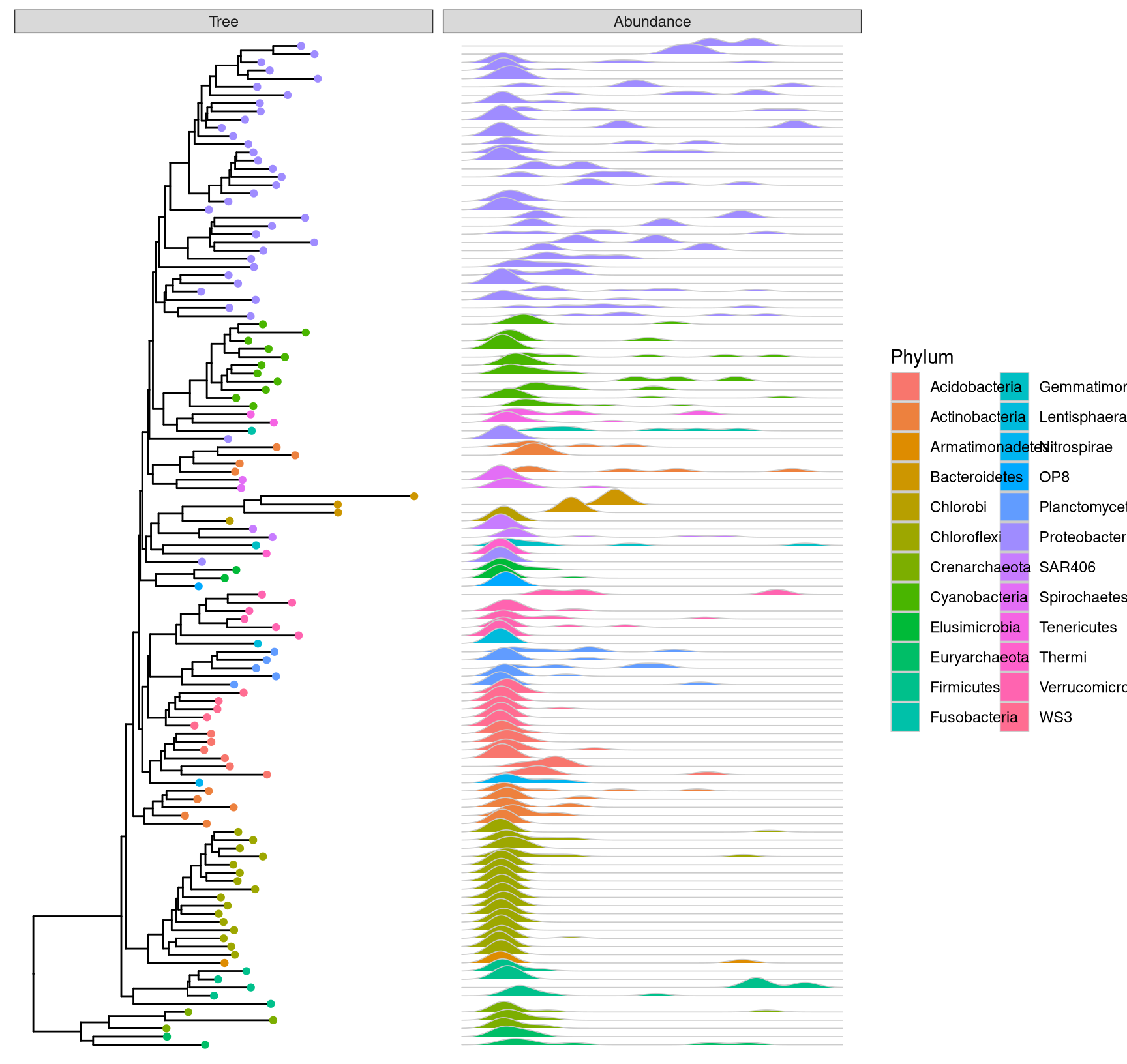

Phylogenetic tree with OTU abundance densities. Tips were colored by Phylum and corresponding abundance across different samples were visualized as density ridgelines and sorted according to the tree structure.

Figure 9.4: Phylogenetic tree with OTU abundance densities. Tips were colored by Phylum and corresponding abundance across different samples were visualized as density ridgelines and sorted according to the tree structure.

This example uses microbiome data that provided in phyloseq package and density ridgeline is employed to visualize species abundance data. The geom_facet layer automatically re-arranges the abundance data according to the tree structure, visualizes the data using the specify geom function, i.e. geom_density_ridges, and aligns the density curves with the tree as demonstrated in Fig. . Note that data stored in the phyloseq object is visible to ggtree and can be used directly in tree visualization (Phylum was used to color tips and density ridgelines in this example). The source code of this example was firstly published in Supplemental File of (Yu et al. 2018).

9.2 ggtree for dendrograms

A dendrogram is a tree diagram to display hierachical clustering and classification/regression trees.

We can calculate a hierachical clustering using the function hclust

hc <- hclust(dist(mtcars))
hc

## 
## Call:
## hclust(d = dist(mtcars))
## 
## Cluster method   : complete 
## Distance         : euclidean 
## Number of objects: 32

The hclust object describes the tree produced by the clustering process. It can be converted to dendrogram object, which stores the tree as deeply-nested lists.

den <- as.dendrogram(hc)
den

## 'dendrogram' with 2 branches and 32 members total, at height 425.3447

The ggtree package supports most of the hierarchical clustering objects defined in the R community, including hclust and dendrogram as well as agnes, diana and twins that defined in the cluster package. Users can use ggtree(object) to display its tree structure, and user other layers and utilities to customize the graph and of course add annotation to the tree.

ggtree provides layout_dendrogram to layout the tree top down, and theme_dendrogram to display tree height (similar to theme_tree2 for phylogenetic tree) as demonstrated in Figure 9.5.

clus <- cutree(hc, 4)
g <- split(names(clus), clus)

p <- ggtree(hc, linetype='dashed')
clades <- sapply(g, function(n) MRCA(p, n))

p <- groupClade(p, clades, group_name='subtree') + aes(color=subtree)

d <- data.frame(label = names(clus), 
                  cyl = mtcars[names(clus), "cyl"])

p %<+% d + 
  layout_dendrogram() + 
  geom_tippoint(size=5, shape=21, aes(fill=factor(cyl), x=x+.5), color='black') + 
  geom_tiplab(aes(label=cyl), size=3, hjust=.5, color='black') +
  geom_tiplab(angle=90, hjust=1, offset=-10, show.legend=F) + 
  scale_color_brewer(palette='Set1', breaks=1:4) +
  theme_dendrogram(plot.margin=margin(6,6,80,6)) +
  theme(legend.position=c(.9, .6))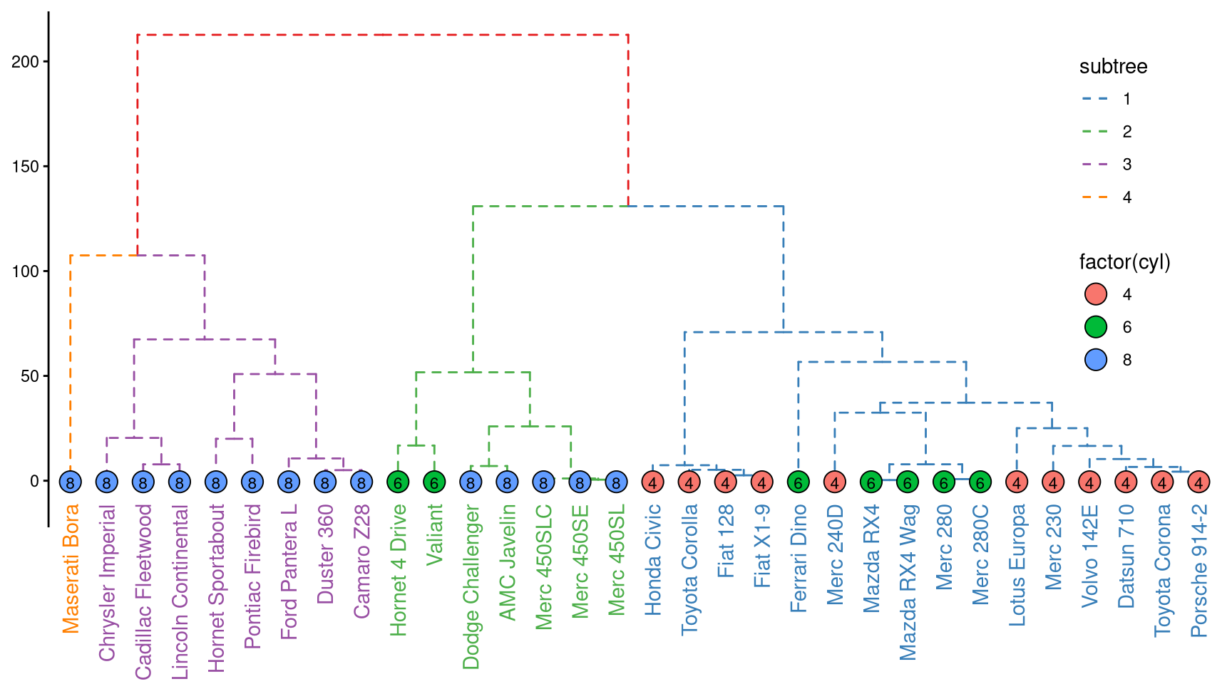

Figure 9.5: Visualizing dendrogram.

9.3 ggtree for tree graph

treeio supports converting tree graph (as an igraph object) to phylo object and ggtree supports directly visualizing tree graph as demonstrated in Figure 9.6.

library(igraph)
g <- graph.tree(40, 3)
arrow_size <- unit(rep(c(0, 3), times = c(27, 13)), "mm")
ggtree(g, layout='slanted', arrow = arrow(length=arrow_size)) + 
  geom_point(size=5, color='steelblue', alpha=.6) + 
  geom_tiplab(hjust=.5,vjust=2) + layout_dendrogram()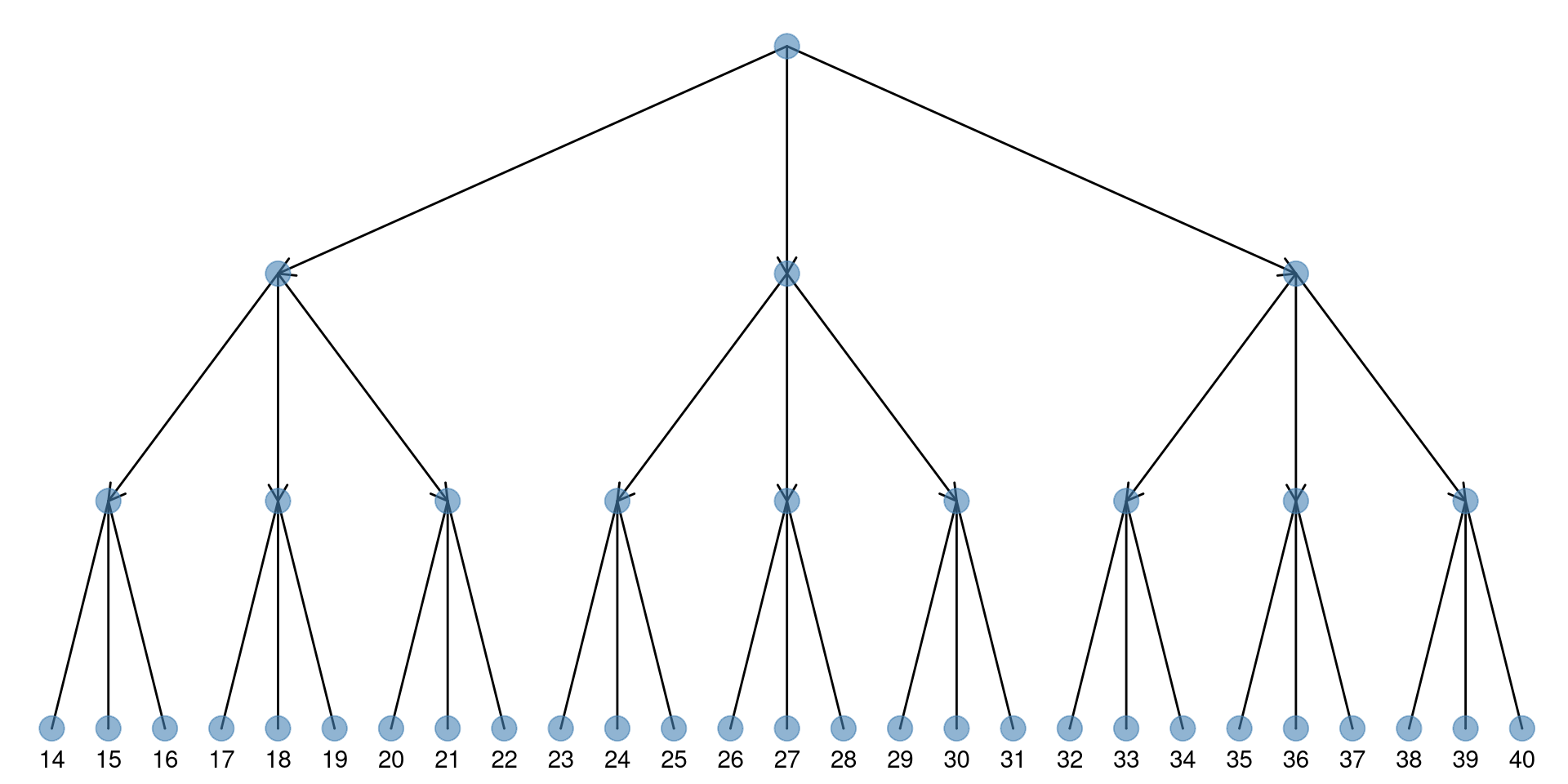

Figure 9.6: Visualizing tree graph.

9.4 ggtree for other tree-like structure

The ggtree package can be used to visualize any data in hierachical structure. Here, we use the GNI (Gross National Income) numbers in 2014 as an example. After preparing an edge list, that is a matrix or data frame that contains two columns indicating the relationship of parent and child nodes, we can use as.phylo provided by treeio to convert the edge list to a phylo object. Then it can be visualized using ggtree with associated data. In this example, the population was used to scale the size of circle points for each country.

library(treeio)
library(ggplot2)
library(ggtree)

data("GNI2014", package="treemap")
n <- GNI2014[, c(3,1)]
n[,1] <- as.character(n[,1])
n[,1] <- gsub("\\s\\(.*\\)", "", n[,1])

w <- cbind("World", as.character(unique(n[,1])))

colnames(w) <- colnames(n)
edgelist <- rbind(n, w)

y <- as.phylo(edgelist)
ggtree(y, layout='circular') %<+% GNI2014 + 
    aes(color=continent) + geom_tippoint(aes(size=population), alpha=.6) + 
    geom_tiplab(aes(label=country), offset=.1) +
    theme(plot.margin=margin(60,60,60,60))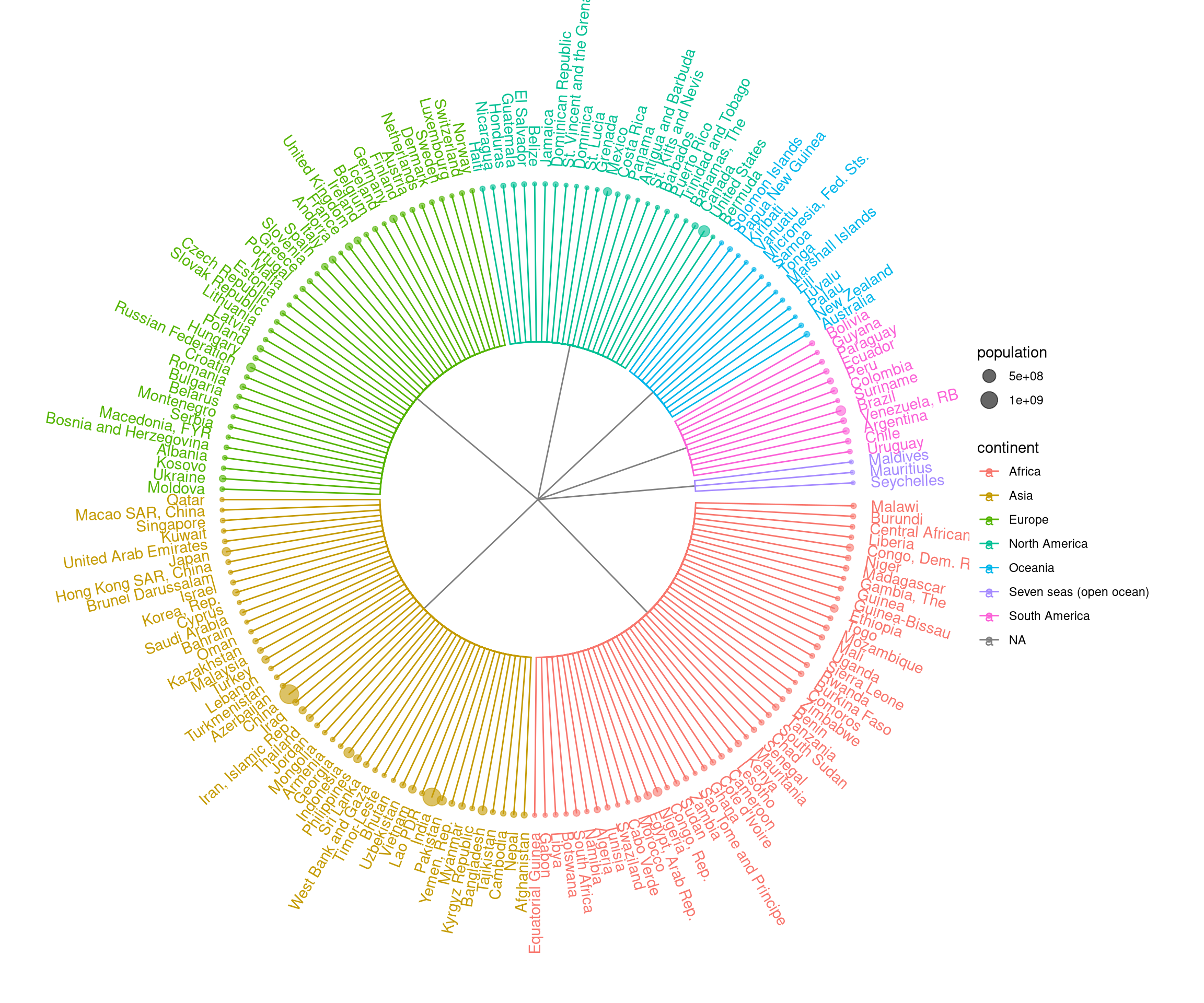

Figure 9.7: Visualizing data in hierachical structure.

References

Callahan, Benjamin J., Paul J. McMurdie, Michael J. Rosen, Andrew W. Han, Amy Jo A. Johnson, and Susan P. Holmes. 2016. “DADA2: High-Resolution Sample Inference from Illumina Amplicon Data.” Nature Methods 13 (7): 581–83. https://doi.org/10.1038/nmeth.3869.

Kuczynski, Justin, Jesse Stombaugh, William Anton Walters, Antonio González, J. Gregory Caporaso, and Rob Knight. 2011. “Using QIIME to Analyze 16S rRNA Gene Sequences from Microbial Communities.” Current Protocols in Bioinformatics / Editoral Board, Andreas D. Baxevanis ... [et Al.] CHAPTER (December): Unit10.7. https://doi.org/10.1002/0471250953.bi1007s36.

Kunin, Victor, and Philip Hugenholtz. 2010. “PyroTagger : A Fast , Accurate Pipeline for Analysis of rRNA Amplicon Pyrosequence Data.” The Open Journal, 1–8. http://www.theopenjournal.org/toj_articles/1.

Schloss, Patrick D., Sarah L. Westcott, Thomas Ryabin, Justine R. Hall, Martin Hartmann, Emily B. Hollister, Ryan A. Lesniewski, et al. 2009. “Introducing Mothur: Open-Source, Platform-Independent, Community-Supported Software for Describing and Comparing Microbial Communities.” Applied and Environmental Microbiology 75 (23): 7537–41. https://doi.org/10.1128/AEM.01541-09.

Yu, Guangchuang, Tommy Tsan-Yuk Lam, Huachen Zhu, and Yi Guan. 2018. “Two Methods for Mapping and Visualizing Associated Data on Phylogeny Using Ggtree.” Molecular Biology and Evolution 35 (12): 3041–3. https://doi.org/10.1093/molbev/msy194.