Chapter 6 Visual Exploration of Phylogenetic Tree
The ggtree supports many ways of manipulating the tree visually, including viewing selected clade to explore large tree (Figure 6.1), taxa clustering (Figure 6.5), rotating clade or tree (Figure 6.6B and 6.8), zoom out or collapsing clades (Figure 6.3A and 6.2), etc.. Details tree manipulation functions are summarized in Table 6.1.
| Function | Descriptiotn |
|---|---|
| collapse | collapse a selecting clade |
| expand | expand collapsed clade |
| flip | exchange position of 2 clades that share a parent node |
| groupClade | grouping clades |
| groupOTU | grouping OTUs by tracing back to most recent common ancestor |
| identify | interactive tree manipulation |
| rotate | rotating a selected clade by 180 degree |
| rotate_tree | rotating circular layout tree by specific angle |
| scaleClade | zoom in or zoom out selecting clade |
| open_tree | convert a tree to fan layout by specific open angle |
6.1 Viewing Selected Clade
A clade is a monophyletic group that contains a single ancestor and all of its descendants. We can visualize a specific selected clade via the viewClade function as demonstrated in Figure 6.1B. Another similar function is gzoom which plots the tree with selected clade side by side. These two functions are developed to explore large tree.
library(ggtree)
nwk <- system.file("extdata", "sample.nwk", package="treeio")
tree <- read.tree(nwk)
p <- ggtree(tree) + geom_tiplab()
viewClade(p, MRCA(p, "I", "L"))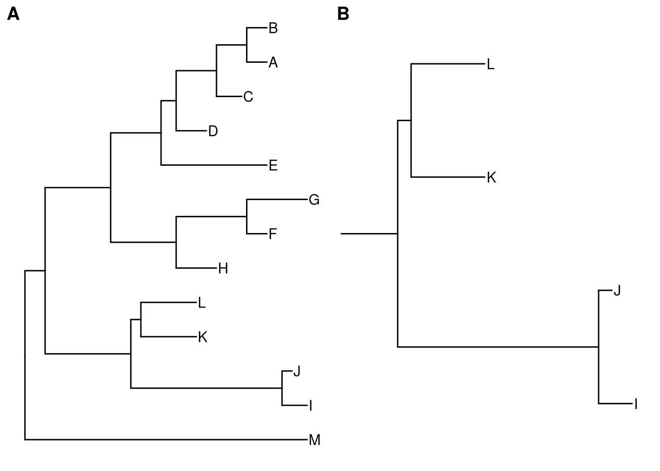
Figure 6.1: Viewing a selected clade of a tree. An example tree used to demonstrate how ggtree support exploring or manipulating phylogenetic tree visually (A). The ggtree supports visualizing selected clade (B). A clade can be selected by specifying a node number or determined by most recent common ancestor of selected tips.
Some of the functions, e.g. viewClade, work with clade and accept a parameter of internal node number. To get the internal node number, user can use MRCA() function (as in Figure 6.1) by providing two taxa names. The function will return node number of input taxa’s most recent common ancestor (MRCA). It works with tree and graphic (i.e. ggtree() output) object. tidytree also provide MRCA function to extract information of MRCA node (see details in session 2.1.3).
6.2 Scaling Selected Clade
The ggtree provides another option to zoom out (or compress) these clades via the scaleClade function. In this way, we retain the topology and branch lengths of compressed clades. This helps to save the space to highlight those clades of primary interest to the study.
tree2 <- groupClade(tree, c(17, 21))
p <- ggtree(tree2, aes(color=group)) + theme(legend.position='none') +
  scale_color_manual(values=c("black", "firebrick", "steelblue"))
scaleClade(p, node=17, scale=.1) 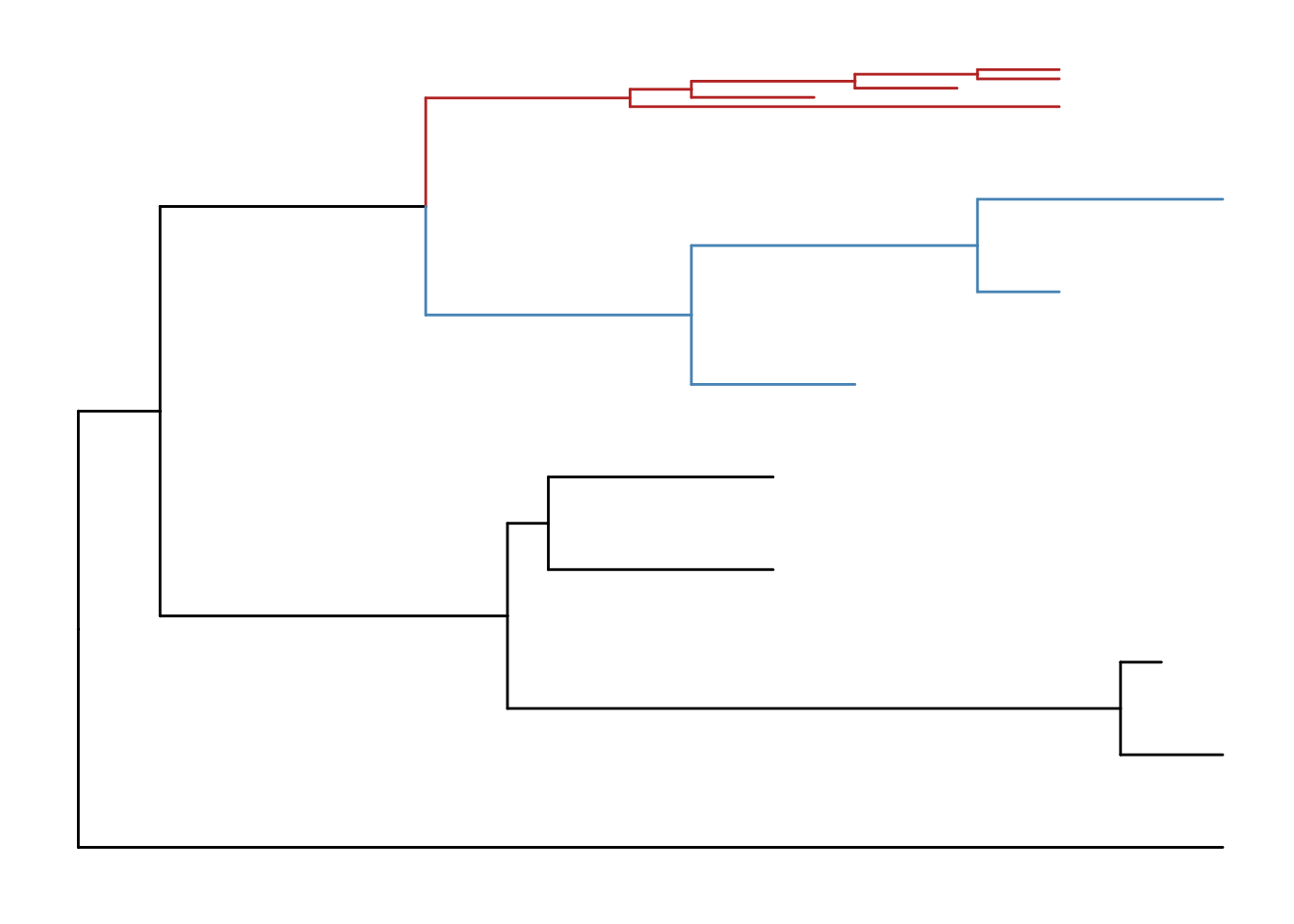
Figure 6.2: Scaling selected clade. Clades can be zoom in (if scale > 1) to highlight or zoom out to save space.
If users want to emphasize important clades, they can use scaleClade function with scale parameter larger than 1. Then the selected clade will be zoomed in. Users can also use groupClade to select clades and color them with different colors as shown in Figure 6.2.
6.3 Collapsing and Expanding Clade
It is a common practice to prune or collapse clades so that certain aspects of a tree can be emphasized. The ggtree supports collapsing selected clades using the collapse function as shown in Figure 6.3A.
p2 <- p %>% collapse(node=21) +
  geom_point2(aes(subset=(node==21)), shape=21, size=5, fill='green')
p2 <- collapse(p2, node=23) +
  geom_point2(aes(subset=(node==23)), shape=23, size=5, fill='red')
print(p2)
expand(p2, node=23) %>% expand(node=21)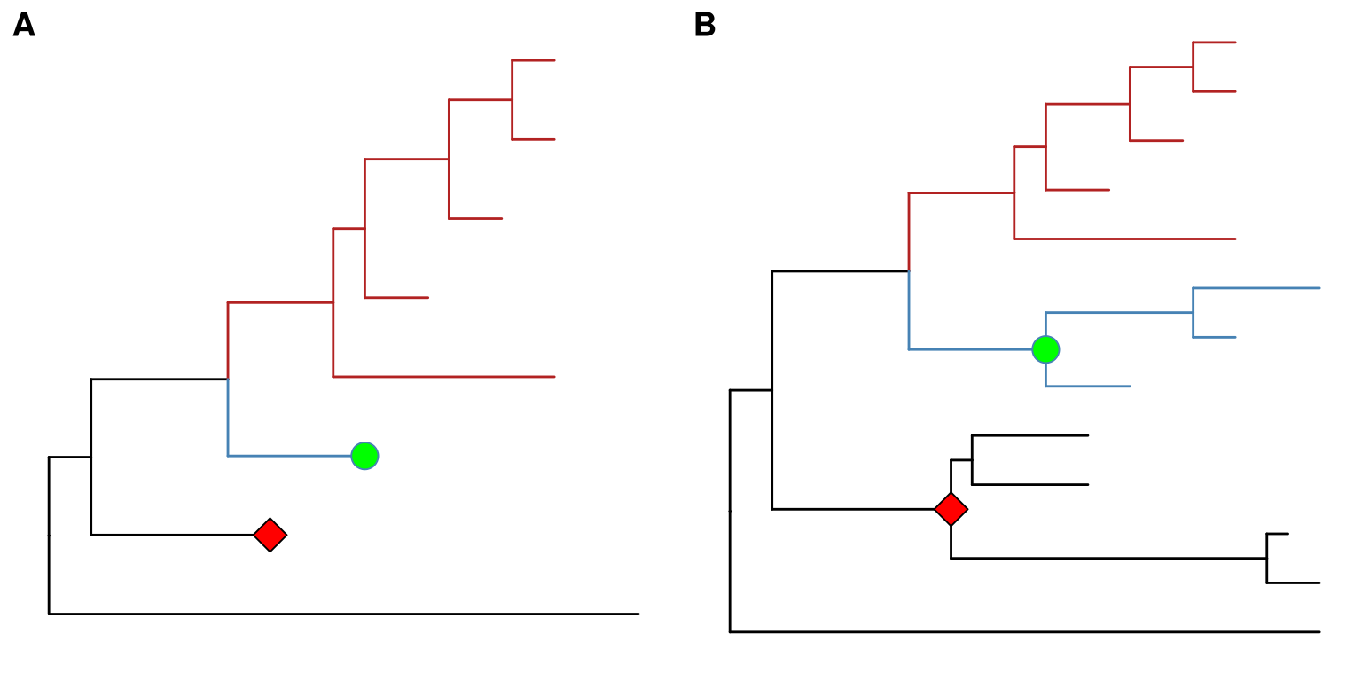
Figure 6.3: Collapsing selected clades and expanding collapsed clades. Clades can be selected to collapse (A) and the collapsed clades can be expanded back (B) if necessary as ggtree stored all information of species relationships. Green and red symbols were displayed on the tree to indicate the collapsed clades.
Here two clades were collapsed and labelled by green circle and red square symbolic points. Collapsing is a common strategy to collapse clades that are too large for displaying in full or are not primary interest of the study. In ggtree, we can expand (i.e., uncollapse) the collapsed branches back with expand function to show details of species relationships as demonstrated in Figure 6.3B.
Triangles are often used to represent the collapsed clade and ggtree also supports it. The collapse function provides a “mode” parameter, which by default is “none” and the selected clade was collapsed as a “tip”. User can specify mode to “max” (Figure 6.4A), “min” (Figure 6.4B) and “mixed” (Figure 6.4C).
p2 <- p + geom_tiplab()
node <- 21
collapse(p2, node, 'max') %>% expand(node)
collapse(p2, node, 'min') %>% expand(node)
collapse(p2, node, 'mixed') %>% expand(node)
We can pass additional parameter to set the color and transparency of the triangles (Figure 6.4D).
collapse(p, 21, 'mixed', fill='steelblue', alpha=.4) %>%
  collapse(23, 'mixed', fill='firebrick', color='blue')
We can combine scaleClade with collapse to zoom in/out of the triangles (Figure 6.4E).
scaleClade(p, 23, .2) %>% collapse(23, 'min', fill="darkgreen") 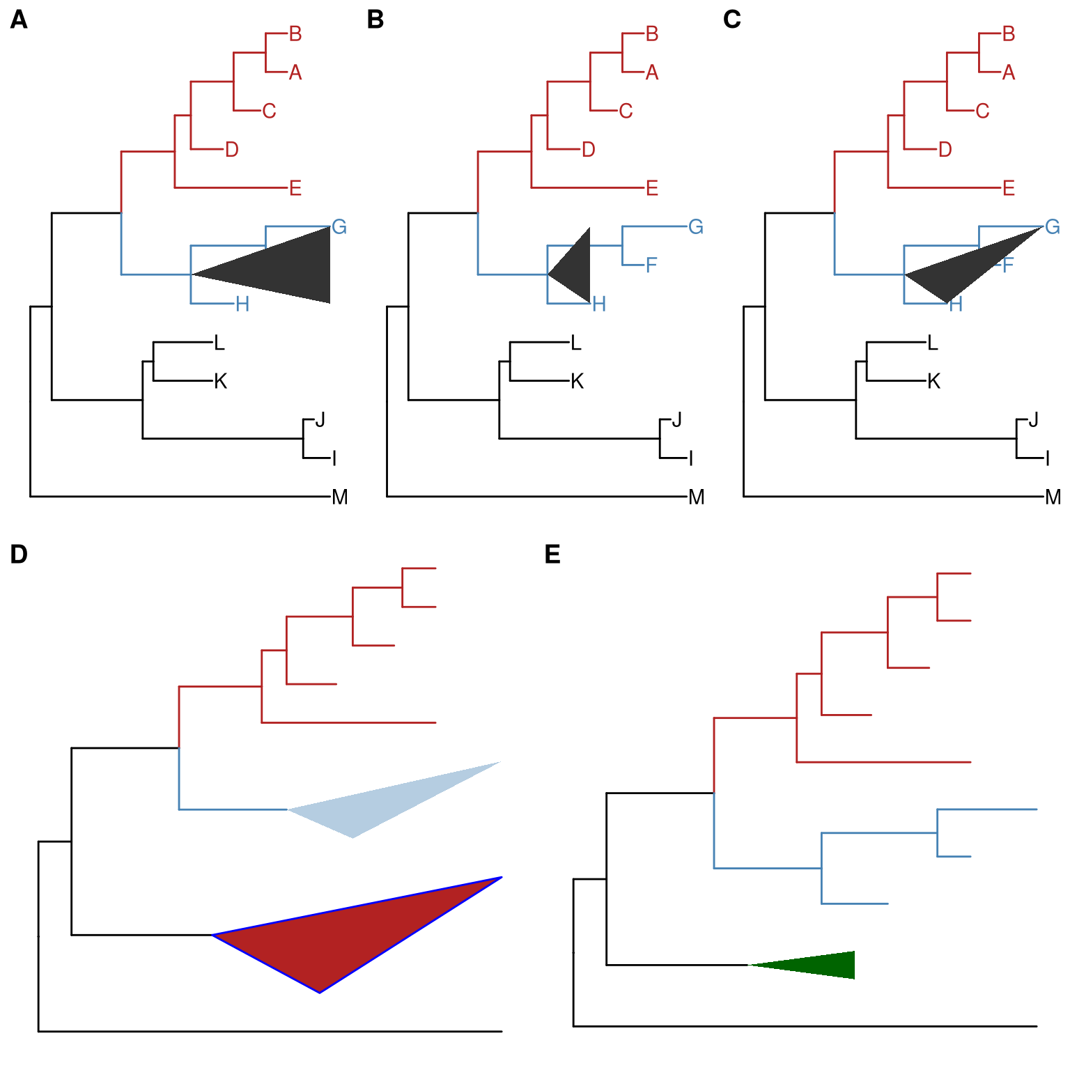
Figure 6.4: Collapse clade as triangle. ‘max’ takes the position of most distant tip (A). ‘min’ takes the position of closest tip (B). ‘mixed’ takes the positions of both closest and distant tips (C), which looks more like the shape of the clade. Set color, fill and alpha of the triangles (D). Combine with scaleClade to zoom out triangle to save space (E).
6.4 Grouping Taxa
The groupClade function assigns the branches and nodes under different clades into different groups. groupClade accepts an internal node or a vector of internal nodes to cluster clade/clades.
Similarly, groupOTU function assigns branches and nodes to different groups based on user-specified groups of operational taxonomic units (OTUs) that are not necessarily within a clade, but can be monophyletic (clade), polyphyletic or paraphyletic. It accepts a vector of OTUs (taxa name) or a list of OTUs and will trace back from OTUs to their most recent common ancestor (MRCA) and cluster them together as demonstrated in Figure 6.5.
A phylogenetic tree can be annotated by mapping different line type, size, color or shape to the branches or nodes that have been assigned to different groups.
data(iris)
rn <- paste0(iris[,5], "_", 1:150)
rownames(iris) <- rn
d_iris <- dist(iris[,-5], method="man")

tree_iris <- ape::bionj(d_iris)
grp <- list(setosa     = rn[1:50],
            versicolor = rn[51:100],
            virginica  = rn[101:150])

p_iris <- ggtree(tree_iris, layout = 'circular', branch.length='none')
groupOTU(p_iris, grp, 'Species') + aes(color=Species) +
  theme(legend.position="right")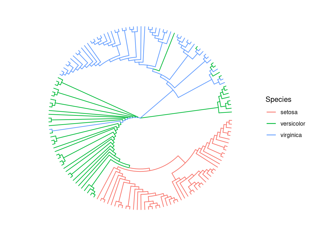
Figure 6.5: Grouping OTUs. OTU clustering based on their relationships. Selected OTUs and their ancestors upto MRCA will be clustered together.
We can grouping taxa at tree level. The following code will produce identical figure of Figure 6.5 (see more details described at session 2.2.3).
tree_iris <- groupOTU(tree_iris, grp, "Species")
ggtree(tree_iris, aes(color=Species), layout = 'circular', branch.length = 'none') +
  theme(legend.position="right")
6.5 Exploring tree structure
To facilitate exploring the tree structure, ggtree supports rotating selected clade by 180 degree using the rotate function (Figure 6.6B). Position of immediate descendant clades of internal node can be exchanged via flip function (Figure 6.6C).
p1 <- p + geom_point2(aes(subset=node==16), color='darkgreen', size=5)
p2 <- rotate(p1, 17) %>% rotate(21)
flip(p2, 17, 21)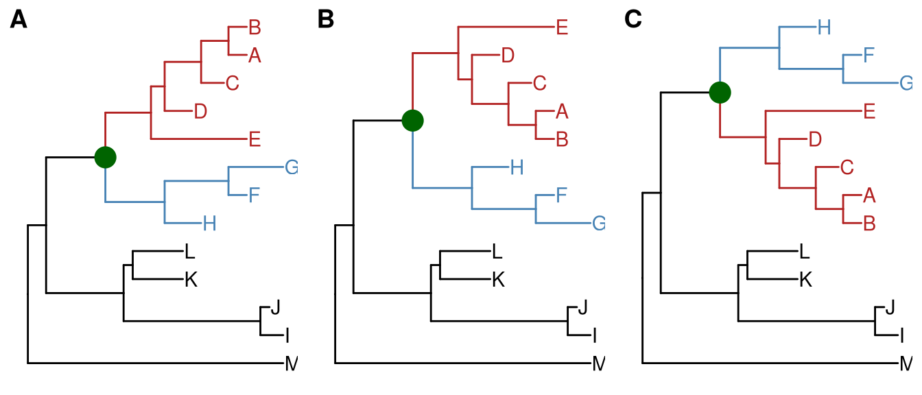
Figure 6.6: Exploring tree structure. A clade (indicated by darkgreen circle) in a tree (A) can be rotated by 180° (B) and the positions of its immediate descedant clades (colored by blue and red) can be exchanged (C).
Most of the tree manipulation functions are working on clades, while ggtree also provides functions to manipulate a tree, including open_tree to transform a tree in either rectangular or circular layout to fan layout, and rotate_tree function to rotate a tree for specific angle in both circular or fan layouts, as demonstrated in Figure 6.7 and 6.8.
p3 <- open_tree(p, 180) + geom_tiplab()
print(p3)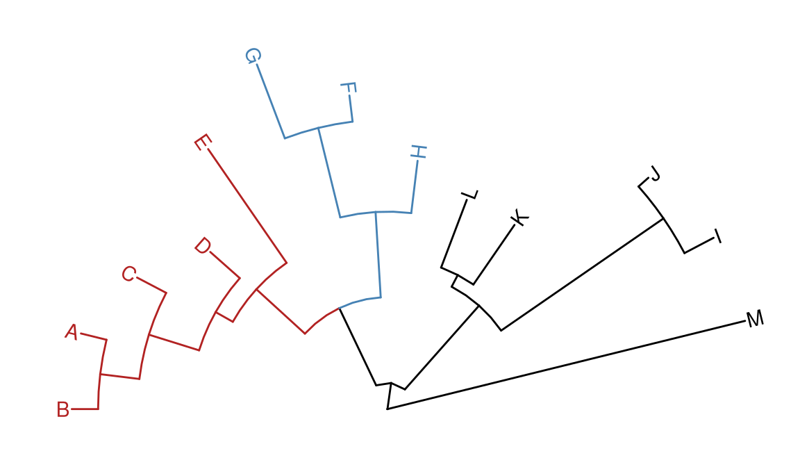
Figure 6.7: Transforming a tree to fan layout. A tree can be transformed to fan layout by open_tree with specific angle parameter.
rotate_tree(p3, 180)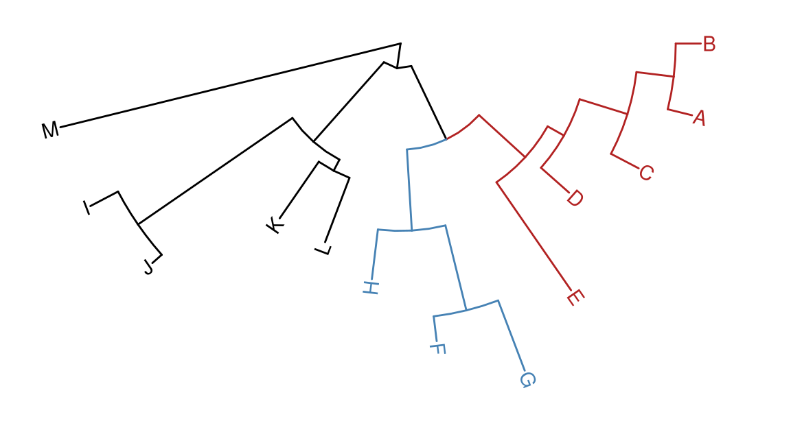
Figure 6.8: Rotating tree. A circular/fan layout tree can be rotated by any specific angle.
The following example traverse all the internal nodes and rotate them one by one (Figure 6.9).
set.seed(2016-05-29)
x <- rtree(50)
p <- ggtree(x) + geom_tiplab()
for (n in reorder(x, 'postorder')$edge[,1] %>% unique) {
    p <- rotate(p, n)
    print(p + geom_point2(aes(subset=(node == n)), color='red'))
}
Figure 6.9: Traverse and rotate all clades.
set.seed(123)
tr <- rtree(50)
p <- ggtree(tr, layout='circular') + geom_tiplab()

for (angle in seq(0, 270, 10)) {
    print(open_tree(p, angle=angle) + ggtitle(paste("open angle:", angle)))
}
Figure 6.10 demonstrates the usage of open_tree with different open angles.
Figure 6.10: Open tree with different angles.
Figure 6.11 illustrates rotating tree with different angles.
for (angle in seq(0, 270, 10)) {
    print(rotate_tree(p, angle) + ggtitle(paste("rotate angle:", angle)))
}
Figure 6.11: Rotate tree with different angles.
Interactive tree manipulation is also possible via identify methods13.
6.6 Summary
The ggtree provides a set of functions to allow visually manipulating phylogenetic tree and exploring tree structure with associated data.